Page 490 - Maxwell House

470 APPENDIX

div = + + (A.19)

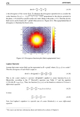
is the divergence of this vector field. To illustrate the divergence operation let us consider the
scalar function (, ) = −1/� + + ( − 0.1) proportional to the electric potential in
2
2
2
the plane z = 0 created by a positive point-size static charge at the point z = 0.1. Then the electric
field vector can be found as = grad (blue arrows in Figure A11). The equipotential line of
divergence is illustrated by black circle.

Figure A11 Divergence function plot (black equipotential lines)

Laplace Operator
2
Assume that some vector field can be represented as = grad where (, , ) is a scalar .
Then the divergence of such field is equal to

2 2 2

div = div(grad) = + + (A.20)
2 2 2
This is the scalar Laplace’s operator div(grad) applied to scalar function (, , ).
rd
Meanwhile, according to the 3 Maxwell’s equation (see Table 1.7 and the equation
(1.32)) div = / . Thus, the function (, , ) can be found as a solution of Poisson’s
0

differential equation
2 2 2

+ + = (, , )/ (A.21)
2 2 2 0
in areas
2
2
2

+ + = 0 (A.22)
2 2 2
Note that Laplace’s equation is a special case of scalar Helmholtz’s or wave differential
equation
2 The reader can find more information about such fields in the sections of Chapter 4.