Page 123 - Mechatronics with Experiments

CLOSED LOOP CONTROL 109
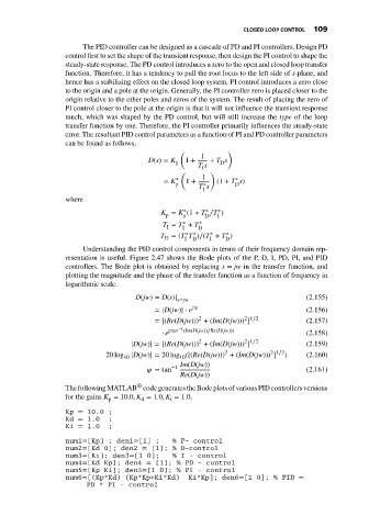
The PID controller can be designed as a cascade of PD and PI controllers. Design PD
control first to set the shape of the transient response, then design the PI control to shape the
steady-state response. The PD control introduces a zero to the open and closed loop transfer
function. Therefore, it has a tendency to pull the root locus to the left side of s-plane, and
hence has a stabilizing effect on the closed loop system. PI control introduces a zero close
to the origin and a pole at the origin. Generally, the PI controller zero is placed closer to the
origin relative to the other poles and zeros of the system. The result of placing the zero of
PI control closer to the pole at the origin is that it will not influence the transient response
much, which was shaped by the PD control, but will still increase the type of the loop
transfer function by one. Therefore, the PI controller primarily influences the steady-state
error. The resultant PID control parameters as a function of PI and PD controller parameters
can be found as follows,
( )
1
D(s) = K p 1 + + T s
D
T s
I
( )
∗ 1 ∗
= K 1 + (1 + T s)
p ∗ D
T s
I
where
∗
∗
∗
K = K (1 + T ∕T )
p
p
I
D
∗
T = T + T D ∗
I
I
∗
∗ ∗
∗
T = (T T )∕(T + T )
D
I
D
I
D
Understanding the PID control components in terms of their frequency domain rep-
resentation is useful. Figure 2.47 shows the Bode plots of the P, D, I, PD, PI, and PID
controllers. The Bode plot is obtained by replacing s = jw in the transfer function, and
plotting the magnitude and the phase of the transfer function as a function of frequency in
logarithmic scale.
(2.155)
D(jw) = D(s)| s=jw
= |D(jw)| ⋅ e jψ (2.156)
2
2 1∕2
= [(Re(D(jw))) + (Im(D(jw))) ] (2.157)
⋅ e j tan −1 (Im(D(jw))∕Re(D(jw))) (2.158)
2
2 1∕2
|D(jw)| = [(Re(D(jw))) + (Im(D(jw))) ] (2.159)
2 1∕2
2
20 log |D(jw)| = 20 log ([(Re(D(jw))) + (Im(D(jw))) ] ) (2.160)
10
10
Im(D(jw))
−1
=tan (2.161)
Re(D(jw))
®
The following MATLAB code generates the Bode plots of various PID controllers versions
for the gains K = 10.0, K = 1.0, K = 1.0,
d
p
i
Kp = 10.0 ;
Kd = 1.0 ;
Ki = 1.0 ;
num1=[Kp] ; den1=[1] ; % P- control
num2=[Kd 0]; den2 = [1]; % D-control
num3=[Ki]; den3=[1 0]; % I - control
num4=[Kd Kp]; den4 = [1]; % PD - control
num5=[Kp Ki]; den5=[1 0]; % PI - control
num6=[(Kp*Kd) (Kp*Kp+Ki*Kd) Ki*Kp]; den6=[1 0]; % PID =
PD * PI - control