Page 199 - Servo Motors and Industrial Control Theory -

196 Appendix B

Assume the following numerical values for the parameters shown in the dia-
gram are,
R1 10 Kohms=
R2 = 5 Kohms
R3 = 50 Kohms
R4 10 Kohms=
R5 = 2 Kohms
C1 0.0000002 Farad=
C2 = 0.0000001 Farad
First derive the transfer function that relates the output variable (uo) to the in-
put variable (ui), use the classical feedback control theory. Plot the frequency
response of the system and determine the frequency bandwidth of the system.
You should note that capacitors are available in microfarad range and resistors
must be chosen in the range of K-ohms so to prevent excessive current drawn
from the system. You should note that OP-AMPs behave like an instant ampli-
fier and its time delay is very small and for practical applications it can be as-
sumed that it behaves as an amplifier with gain of,
K = R3/R2

Repeat this problem and write the governing differential equations and convert
them to state space form. Find the frequency bandwidth of the output variable
uo with respect to ui.
Discuss the frequency response characteristics of the system derived from the
above mentioned two methods. You should know that the cutoff (corner) fre-
quency occurs when the amplitude ratio drops 3 db below the low frequency
response.
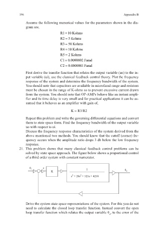
21. This problem shows that many classical feedback control problems can be
solved by state space approach. The figure below shows a proportional control
of a third order system with constant numerator.

θ i e 1
K θ o
3
2
s + 20s + 525s + 4250

Drive the system state space representations of the system. For this you do not
need to calculate the closed loop transfer function. Instead convert the open
loop transfer function which relates the output variable θ , to the error of the
o