Page 642 - Krugmans Economics for AP Text Book_Neat

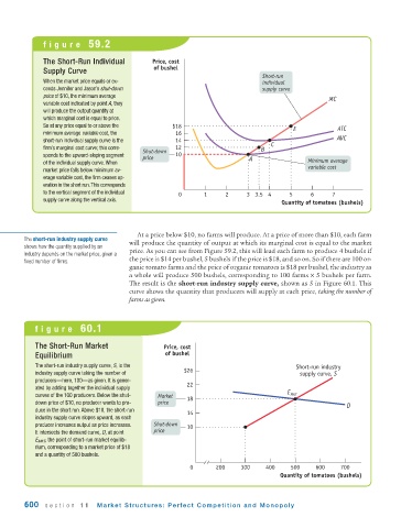
figure 59.2

The Short-Run Individual Price, cost
of bushel
Supply Curve
Short-run
When the market price equals or ex- individual
ceeds Jennifer and Jason’s shut-down supply curve
price of $10, the minimum average
MC
variable cost indicated by point A, they
will produce the output quantity at
which marginal cost is equal to price.
So at any price equal to or above the $18 E ATC
minimum average variable cost, the 16
short-run individual supply curve is the 14 AVC
firm’s marginal cost curve; this corre- 12 C
Shut-down B
sponds to the upward-sloping segment 10
price A
of the individual supply curve. When Minimum average
variable cost
market price falls below minimum av-
erage variable cost, the firm ceases op-
eration in the short run. This corresponds
to the vertical segment of the individual 0 1 2 3 3.5 4 5 6 7
supply curve along the vertical axis.
Quantity of tomatoes (bushels)

At a price below $10, no farms will produce. At a price of more than $10, each farm
The short-run industry supply curve will produce the quantity of output at which its marginal cost is equal to the market
shows how the quantity supplied by an
industry depends on the market price, given a price. As you can see from Figure 59.2, this will lead each farm to produce 4 bushels if
fixed number of firms. the price is $14 per bushel, 5 bushels if the price is $18, and so on. So if there are 100 or-
ganic tomato farms and the price of organic tomatoes is $18 per bushel, the industry as
a whole will produce 500 bushels, corresponding to 100 farms × 5 bushels per farm.
The result is the short-run industry supply curve, shown as S in Figure 60.1. This
curve shows the quantity that producers will supply at each price, taking the number of
farms as given.

figure 60.1

The Short-Run Market Price, cost
Equilibrium of bushel
The short-run industry supply curve, S, is the Short-run industry
industry supply curve taking the number of $26 supply curve, S
producers—here, 100—as given. It is gener- 22
ated by adding together the individual supply
E
curves of the 100 producers. Below the shut- Market 18 MKT
down price of $10, no producer wants to pro- price
D
duce in the short run. Above $10, the short-run 14
industry supply curve slopes upward, as each
producer increases output as price increases. Shut-down 10
It intersects the demand curve, D, at point price
E MKT , the point of short-run market equilib-
rium, corresponding to a market price of $18
and a quantity of 500 bushels.
0 200 300 400 500 600 700
Quantity of tomatoes (bushels)

600 section 11 Market Structures: Perfect Competition and Monopoly