Page 645 - Krugmans Economics for AP Text Book_Neat

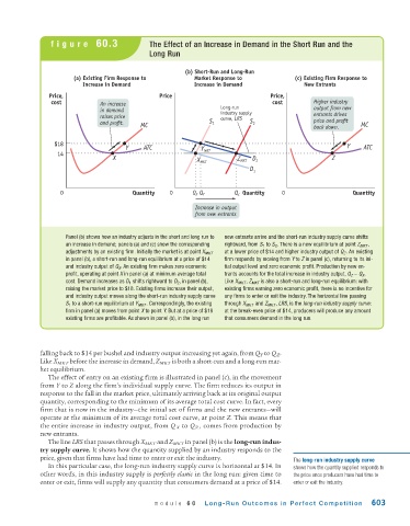
figure 60.3 The Effect of an Increase in Demand in the Short Run and the
Long Run

(b) Short-Run and Long-Run
(a) Existing Firm Response to Market Response to (c) Existing Firm Response to
Increase in Demand Increase in Demand New Entrants
Price, Price Price,
cost An increase cost Higher industry
in demand Long-run output from new
industry supply
raises price curve, LRS entrants drives
and profit. MC S 1 S 2 price and profit MC
back down.
$18
Y ATC Y Y ATC
14 MKT
X X MKT Z MKT D 2 Z
D 1

0 Quantity 0 Q X Q Y Q Z Quantity 0 Quantity

Increase in output
from new entrants

Panel (b) shows how an industry adjusts in the short and long run to new entrants arrive and the short-run industry supply curve shifts
an increase in demand; panels (a) and (c) show the corresponding rightward, from S 1 to S 2 . There is a new equilibrium at point Z MKT ,
adjustments by an existing firm. Initially the market is at point X MKT at a lower price of $14 and higher industry output of Q Z . An existing
in panel (b), a short-run and long-run equilibrium at a price of $14 firm responds by moving from Y to Z in panel (c), returning to its ini-
and industry output of Q X . An existing firm makes zero economic tial output level and zero economic profit. Production by new en-
profit, operating at point X in panel (a) at minimum average total trants accounts for the total increase in industry output, Q Z − Q X .
cost. Demand increases as D 1 shifts rightward to D 2 , in panel (b), Like X MKT , Z MKT is also a short-run and long-run equilibrium: with
raising the market price to $18. Existing firms increase their output, existing firms earning zero economic profit, there is no incentive for
and industry output moves along the short-run industry supply curve any firms to enter or exit the industry. The horizontal line passing
S 1 to a short-run equilibrium at Y MKT . Correspondingly, the existing through X MKT and Z MKT , LRS, is the long-run industry supply curve:
firm in panel (a) moves from point X to point Y. But at a price of $18 at the break-even price of $14, producers will produce any amount
existing firms are profitable. As shown in panel (b), in the long run that consumers demand in the long run.

falling back to $14 per bushel and industry output increasing yet again, from Q Y to Q Z .
Like X MKT before the increase in demand, Z MKT is both a short-run and a long-run mar-
ket equilibrium.
The effect of entry on an existing firm is illustrated in panel (c), in the movement
from Y to Z along the firm’s individual supply curve. The firm reduces its output in
response to the fall in the market price, ultimately arriving back at its original output
quantity, corresponding to the minimum of its average total cost curve. In fact, every
firm that is now in the industry—the initial set of firms and the new entrants—will
operate at the minimum of its average total cost curve, at point Z. This means that
the entire increase in industry output, from Q X to Q Z , comes from production by
new entrants.
The line LRS that passes through X MKT and Z MKT in panel (b) is the long-run indus-
try supply curve. It shows how the quantity supplied by an industry responds to the
price, given that firms have had time to enter or exit the industry. The long-run industry supply curve
In this particular case, the long-run industry supply curve is horizontal at $14. In shows how the quantity supplied responds to
other words, in this industry supply is perfectly elastic in the long run: given time to the price once producers have had time to
enter or exit, firms will supply any quantity that consumers demand at a price of $14. enter or exit the industry.

module 60 Long-Run Outcomes in Perfect Competition 603