Page 643 - Krugmans Economics for AP Text Book_Neat

The market demand curve, labeled D in Figure 60.1, crosses the short-run industry
There is a short-run market
supply curve at E MKT , corresponding to a price of $18 and a quantity of 500 bushels.
equilibrium when the quantity supplied
Point E MKT is a short-run market equilibrium: the quantity supplied equals the equals the quantity demanded, taking the
quantity demanded, taking the number of farms as given. But the long run may look number of producers as given.
quite different because in the long run farms may enter or exit the industry.

The Long-Run Industry Supply Curve
Suppose that in addition to the 100 farms currently in the organic tomato business,
there are many other potential organic tomato farms. Suppose also that each of these
potential farms would have the same cost curves as existing farms, like the one owned
by Jennifer and Jason, upon entering the industry. Section 11 Market Structures: Perfect Competition and Monopoly
When will additional farms enter the industry? Whenever existing farms are making
a profit—that is, whenever the market price is above the break-even price of $14 per
bushel, the minimum average total cost of production. For example, at a price of $18
per bushel, new farms will enter the industry.
What will happen as additional farms enter the industry? Clearly, the quantity sup-
plied at any given price will increase. The short-run industry supply curve will shift to the
right. This will, in turn, alter the market equilibrium and result in a lower market price.
Existing farms will respond to the lower market price by reducing their output, but the
total industry output will increase because of the larger number of farms in the industry.
Figure 60.2 illustrates the effects of this chain of events on an existing farm and on
the market; panel (a) shows how the market responds to entry, and panel (b) shows

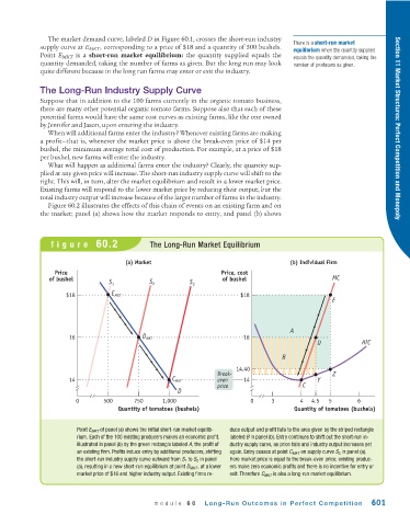
figure 60.2 The Long-Run Market Equilibrium

(a) Market (b) Individual Firm
Price Price, cost
of bushel of bushel MC
S 1 S 2 S 3
$18 E MKT $18
E

A
16 D MKT 16
D ATC

B
14.40
Break- Z
14 C MKT even 14 Y
price C
D
0 500 750 1,000 0 3 4 4.5 5 6
Quantity of tomatoes (bushels) Quantity of tomatoes (bushels)

Point E MKT of panel (a) shows the initial short-run market equilib- duce output and profit falls to the area given by the striped rectangle
rium. Each of the 100 existing producers makes an economic profit, labeled B in panel (b). Entry continues to shift out the short-run in-
illustrated in panel (b) by the green rectangle labeled A, the profit of dustry supply curve, as price falls and industry output increases yet
an existing firm. Profits induce entry by additional producers, shifting again. Entry ceases at point C MKT on supply curve S 3 in panel (a).
the short-run industry supply curve outward from S 1 to S 2 in panel Here market price is equal to the break-even price; existing produc-
(a), resulting in a new short-run equilibrium at point D MKT , at a lower ers make zero economic profits and there is no incentive for entry or
market price of $16 and higher industry output. Existing firms re- exit. Therefore C MKT is also a long-run market equilibrium.

module 60 Long-Run Outcomes in Perfect Competition 601