Page 54 - u4

P2: OSO/OVY
P1: OSO/OVY
GO-01962Smith-v1.cls
UAE-Math-Grade-12-Vol-1-SE-718383-ch4
SECTION 4.4 • •
4-35 QC: OSO/OVY T1: OSO October 25, 2018 17:24 Increasing and Decreasing Functions 245
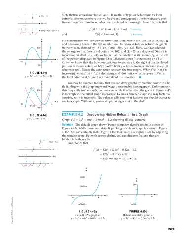
- 0 + Note that the critical numbers (1 and −4) are the only possible locations for local
6(x - 1)
1 extrema. We can see where the two factors and consequently the derivative are posi-
- 0 + tive and negative from the number lines displayed in the margin. From this, note that
(x + 4)
-4
+ 0 - 0 + f (x) > 0 on (− , −4) (1, ) f increasing
f'(x) = 6(x - 1)(x + 4)
-4 1
and f (x) < 0 on (−4, 1). f decreasing.
y
For convenience, we have placed arrows indicating where the function is increasing
and decreasing beneath the last number line. In Figure 4.44a, we redraw the graph
100 in the window defined by −8 ≤ x ≤ 4 and −50 ≤ y ≤ 125. Here, we have selected
the y-range so that the critical points (−4, 102) and (1, −23) are displayed. Since f is
increasing on all of (− , −4), we know that the function is still increasing to the left
x of the portion displayed in Figure 4.44a. Likewise, since f is increasing on all of
-8 4 (1, ), we know that the function continues to increase to the right of the displayed
-50 portion. In Figure 4.44b, we have plotted both y = f(x) (shown in blue) and y = f (x)
(shown in red). Notice the connection between the two graphs. When f (x) > 0,f is
FIGURE 4.44a increasing; when f (x) < 0,f is decreasing and also notice what happens to f (x) at
2
3
y = 2x + 9x − 24x − 10 the local extrema of f. (We’ll say more about this shortly.)
y
You may be tempted to think that you can draw graphs by machine and with a lit-
tle fiddling with the graphing window, get a reasonable looking graph. Unfortunately,
f(x)
100 this frequently isn’t enough. For instance, while it’s clear that the graph in Figure 4.43
is incomplete, the initial graph in example 4.2 has a familiar shape and may look rea-
sonable, but it is incorrect. The calculus tells you what features you should expect to
x see in a graph. Without it, you’re simply taking a shot in the dark.
-8 4
f'(x)
-50

FIGURE 4.44b EXAMPLE 4.2 Uncovering Hidden Behavior in a Graph
y = f(x) and y = f (x) Graph f(x) = 3x + 40x − 0.06x − 1.2x showing all local extrema.
3
2
4
Solution The default graph drawn by our computer algebra system is shown in
Figure 4.45a, while a common default graphing calculator graph is shown in Figure
4.45b. You can certainly make Figure 4.45b look more like Figure 4.45a by adjusting
the window some. But with some calculus, you can discover features that are
hidden in both graphs.
- 0 +
12(x - 0.1)
0.1 First, notice that
- 0 +
3
2
(x + 0.1) f (x) = 12x + 120x − 0.12x − 1.2
-0.1
2
- 0 + = 12(x − 0.01)(x + 10)
(x + 10)
-10 = 12(x − 0.1)(x + 0.1)(x + 10).
- 0 + 0 - 0 +
f'(x)
-10 -0.1 0.1
y
6000 y
10
3000

x -10 10 x
4
Copyright © McGraw-Hill Education y = 3x + 40x − 0.06x − 1.2x y = 3x + 40x − 0.06x − 1.2x
-4
-10
-3000
E
4 . 4
G I F
U
R
G I F
5
a
E
4 . 4
R
U
b
5
Default CAS graph of
Default calculator graph of
3
2
2
4
3
4
263