Page 242 - Linear Models for the Prediction of Animal Breeding Values 3rd Edition

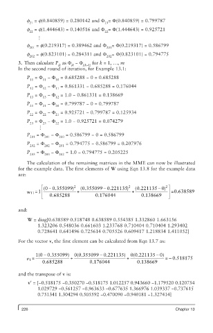
f = f(0.840859) = 0.280142 and F = F(0.840859) = 0.799787
21 21
f = f(1.444643) = 0.140516 and F = F(1.444643) = 0.925721
22 22

= f(0.219317) = 0.389462 and F = F(0.219317) = 0.586799
201 201
f
= f(0.823101) = 0.284311 and F = F(0.823101) = 0.794775
202 202
f
3. Then calculate P as F − F for k = 1, ..., m
jk jk j(k−1)
In the second round of iteration, for Example 13.1:
P = F − F = 0.685288 − 0 = 0.685288
11 11 10
P = F − F = 0.861331 − 0.685288 = 0.176044
12 12 11
P = F − F = 1.0 − 0.861331 = 0.138669
13 13 12
P = F − F = 0.799787 − 0 = 0.799787
21 21 20
P = F − F = 0.925721 − 0.799787 = 0.125934
22 22 21
P = F − F = 1.0 − 0.925721 = 0.074279
23 23 22

P = F − F = 0.586799 − 0 = 0.586799
201 201 200
P = F − F = 0.794775 − 0.586799 = 0.207976
202 202 201
P = F − F = 1.0 − 0.794775 = 0.205225
203 203 202
The calculation of the remaining matrices in the MME can now be illustrated
for the example data. The first elements of W using Eqn 13.8 for the example data
are:

é (0 0.355099) 2 (0.355099 0.221135) 2 (0.221135 0) ù
2
-
-
-
w =1 ê + + ú =0.638589
11
ë 0.685288 0.1776044 0.138669 û
and:
W = diag[0.638589 0.518748 0.638589 0.554385 1.332860 1.663156
1.323206 0.548036 0.661603 1.233768 0.710404 0.710404 1.293402
0.728641 0.641496 0.725614 0.705526 0.609417 1.218834 1.411052]

For the vector v, the first element can be calculated from Eqn 13.7 as:

−
−
−
1(0 0.355099) 0(0.355099 0.221135) 0(0.221135 0)
−
1 v = + + = 0.518175
0.685288 0.1760044 0.138669
and the transpose of v is:
v′ = [−0.518175 −0.350270 −0.518175 1.012257 0.943660 −1.179520 0.120754
1.029729 −0.561257 −0.963633 −0.677635 1.366976 1.039337 −0.737615
0.751341 1.304294 0.505592 −0.470090 −0.940181 −1.327414]

226 Chapter 13