Page 247 - Linear Models for the Prediction of Animal Breeding Values 3rd Edition

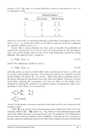
Section 13.2.2, the data for calving difficulty could be represented in an s by
2 contingency table:
Response category
Row Easy calving Difficult calving

1 n n − n
11 1. 11
2 n n − n
21 2. 21

j n n − n
j1 j. j1

s n n − n
s1 s. s1
where the s rows refer to conditions affecting an individual or grouped records. Note
that n or n − n in the above table can be null, as responses in the two categories
i1 i. i1
are mutually exclusive, but n ¹ 0.
i
Assume that a normal function has been used to describe the probability of
response for calving ease. Let y be the vector for observations for the quantitative
1
trait, such as birth weight, and y be the vector of the underlying variable for calving
2
difficulty. The model for trait 1 would be:
y = X b + Z u + e (13.13)
1 1 1 1 1 1
and for the underlying variable for trait 2:

y = X b + Z u + e (13.14)
2 2 2 2 2 2
where b and u are vectors of fixed effect and sire solutions for trait 1, and X and
1 1 1
Z are the usual incidence matrices. The matrices X and Z are incidence matrices
1 2 2
for the liability. The matrix Z = Z and X = X H, where H is an identity matrix if
2 1 2 1
all factors affecting the quantitative traits also affect the liability. However, if certain
fixed effects affecting the quantitative trait have no effect on the liability, H is
obtained by deleting the columns of an identity matrix of appropriate order corre-
sponding to such effects. It is assumed that:
e ⎛ 1 ⎞ ⎛ R 11 R 12 ⎞
var ⎜ e ⎝ 2 ⎟ ⎠ = ⎜ ⎝ R 21 R ⎠ ⎟
22
⎛ u 1 ⎞
var ⎜ ⎝ u ⎠ ⎟ = A ⊗ G (13.15)
2
where G is the genetic covariance matrix for both traits and A is the numerator rela-
tionship matrix.
Let q′ = [b , t, u , n], the vector of location parameters in Eqns 13.13 and 13.14 to be
1 1
estimated, where t = b − bHb and n = u − bu , where b is the residual regression coeffi-
2 1 2 1
cient of the underlying variate on the quantitative trait. The calculation of b is illustrated in
the next section. Since the residual variance of liability is unity, the use of b is necessary to
properly adjust the underlying variate for the effect of the residual covariance between both

Analysis of Ordered Categorical Traits 231