Page 249 - Linear Models for the Prediction of Animal Breeding Values 3rd Edition

Calculating m and the residual regression coefficient

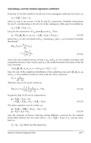
From Eqn 13.14, the model for the jth row of the contingency table may be written as:
y = x′ b + z′ u + e
2j 2j 2 2j 2 2j
where x′ and z′ are vectors j of the X and Z , respectively. Similarly, observations
2j 2j 2 2 .
for trait 1, corresponding to the jth row of the contingency table, may be modelled as:
y = x′ b + z′ u + e
1j 1j 1 1j 1 1j
Let m be the expectation of y given b, u and y . Thus:
j 2j 1j
m = E(y | b , b , u , u , y ) = x′ b + z′ u + E(e | e ) (13.20)
j 2j 1 2 1 2 1j 2j 2 2j 2 2j 1j
given that e is only correlated with e . Assuming e and e are bivariately normally
2j 1j 2j 1j
distributed:
21
E(e | e ) = s e(, ) e ()
2j 1j 2 1j
e1
s
⎛ ⎞
= r 12 ⎜ s e2 ⎟ e
⎝ s e1 ⎠ 1j (13.21)
2 and r are the residual covariance and
ei
where s is the residual variance of trait i, s ei,k ik
correlation between traits i and k, and s is the residual standard deviation of the ith
ei
trait. Similarly:
2
2
var(y | b , b , u , u , y ) = var(e | e ) = s (1 − r )
2j 1 2 1 2 1j 2j 1j e2 12
Since the unit of the conditional distribution of the underlying trait, given b , b , u , u
1 2 1 2
and y is the standard deviation, then from the above equation:
1j,
= 1
e2
s 2
( 1− r )
12
Therefore, Eqn 13.21 can be written as:
⎛ 1 ⎞ 1
E(e | e ) = r 12 ⎜ e = be (13.22)
j 2 j 1 e1 ⎠ ⎟ 2 j 1 j 1
⎝ s 1 − r 12
In general, Eqn 13.20 can be expressed as:
m = X b + Z u + be
2 2 2 2 1
= X b + Z u + b(y − X b − Z u ) (13.23)
2 2 2 2 1 1 1 1 1
The above equation may be written as:
m = X (b − bHb ) + Z (u − bu ) + by *
2 2 1 2 2 1 1
m = X t + Z n + by * (13.24)
2 2 1
with the solutions of factors affecting calving difficulty corrected for the residual
*
*
relationship between the two traits and y = (y − X b − Z u ) or y may be calcu-
1 1 1 1 1 1 1
lated as:
y = y ( − y ), where is the mean of y .
*
y
1 1 1 1 1
Analysis of Ordered Categorical Traits 233