Page 251 - Linear Models for the Prediction of Animal Breeding Values 3rd Edition

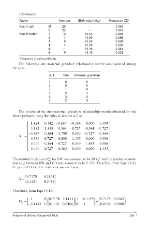
(Continued)
Factor Number Birth weight (kg) Frequency CD a
Sex of calf M 25 – 0.360
F 22 – 0.091
Sire of heifer 1 10 40.55 0.000
2 7 42.99 0.286
3 6 40.53 0.000
4 4 45.38 0.500
5 11 45.46 0.364
6 9 43.43 0.333
a Frequency of calving difficulty.
The following sire–maternal grandsire relationship matrix was assumed among
the sires:
Bull Sire Maternal grandsire

1 0 0
2 0 0
3 1 0
4 2 1
5 3 2
6 2 3

The inverse of the sire–maternal grandsire relationship matrix obtained for the
above pedigree using the rules in Section 2.5 is:

⎡ 1.424 0.182 −0.667 −0.364 0.000 0.000⎤
⎢ − 0.364 − ⎥
7
⎢ 0.182 1.818 0.364 −0.727 0.727 ⎥
− ⎢ 0.667 0.364 1.788 0.000 − 0.727 − 0.364⎥
−1
A = ⎢ ⎥
7
⎢ − 0.364 − 0.727 0.000 1.455 0.000 0.000 ⎥
⎢ 0.000 − 0.364 − 0.727 0.000 1.455 0.000 ⎥
⎢ ⎥
⎣ ⎢ 0.000 − 0.727 − 0.364 0.000 0.000 1.455⎥ ⎦
0
The residual variance (s ) for BW was assumed to be 20 kg and the residual correla-
2
2
e1
tion (r ) between BW and CD was assumed to be 0.459. Therefore, from Eqn 13.20,
12
b equals 0.1155. The matrix G assumed was:
æ0.7178 0.1131 ö
G = ç ÷
è 0.1131 0.0466 ø

Therefore, from Eqn 13.16:

0 7178 0 0302⎞
G = ⎛ 1 0 ⎞ ⎛0 7178 0 1131 1. . . ⎞ ⎛ −0 1155. ⎞ ⎟ ⎠ = ⎛ . . . ⎟
⎟ ⎜
⎜
⎜
⎟ ⎜
c
0 0302 0 0300⎠
⎠ ⎝
⎝
⎠ ⎝0 1131 0 0466 0.
⎝ .
−0 1155 1.
1 1
Analysis of Ordered Categorical Traits 235