Page 248 - Linear Models for the Prediction of Animal Breeding Values 3rd Edition

traits. The use of b can be thought of as correcting calving difficulty for other ‘risk’ factors
affecting calving and, in this example, the birth weight of the calf. Thus Eqn 13.15 may
be written as:
⎛ u 1 ⎞ ⎛ u 1 ⎞
var ⎜ ⎝ u − b u ⎠ ⎟ = ⎜ ⎝ ν ⎟ ⎠ = A ⊗ G c
1
2
where:
I ⎛ 0⎞ ⎛ g gg ⎞ I ⎛ −b I⎞
Gc = ⎜ ⎝ −b II ⎠ ⎝ g 11 gg 12 ⎟ ⎜ 0 I⎠ ⎟ (13.16)
⎟ ⎜
⎠ ⎝
22
21
with g being the elements of G.
ij
Using a Bayesian approach, Foulley et al. (1983) calculated the mode of the pos-
terior density of q by equating the derivatives of the log-posterior density of q to zero.
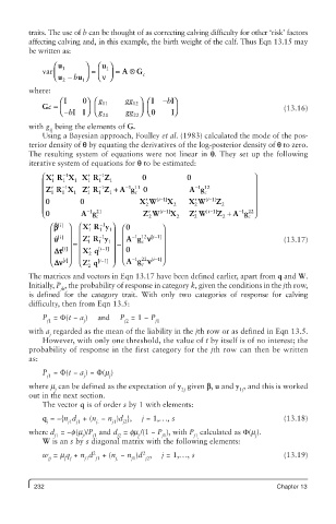
The resulting system of equations were not linear in q. They set up the following
iterative system of equations for q to be estimated:
−
−
′
′
⎛ XR X X R Z 1 0 0 ⎞
1
1
1
1
1
1
1
⎜ ⎟
′
−
−
′
−
−
1 12
111
1
1
⎜ ZR X 1 Z R Z + A g c 0 A g c ⎟
1
1
1
1
1
⎜ [i− 1] [i− 1] ⎟
′
⎜ 0 0 X′ W X 2 X W Z 2 ⎟
2
2 2
⎜ − 121 [i− 1] [i− 1] − 122⎟
′
′
2
⎝ 0 A g c Z W X 2 Z W Z + A g ⎠
c
2
2
2
′
−
1
⎛b ˆ [] i ⎞ ⎛ XR y ⎞ ⎛ 0 ⎞
y
1
1
1
⎜ [] i ⎟ ⎜ − 1 ⎟ ⎜ − 112 [i − 1]⎟
′
]
⎜ ˆ u ⎟ ⎜ ZR y ⎟ ⎜ Ag n ⎟ (13.17)
1
1
c
1
1 ⎟
⎜ [] i ⎟ = ⎜ [i − ] − ⎜ 0 ⎟
′
⎜ Dt ⎟ ⎜ Xq ⎟ ⎜ ⎟
2
1 ⎟
⎜ ⎝ Dn [] i ⎟ ⎠ ⎜ ⎝ Zq [i − ] ⎠ ⎜ ⎝ Ag n [ −1i ]⎟ ⎠
−122
′
c
2
The matrices and vectors in Eqn 13.17 have been defined earlier, apart from q and W.
Initially, P , the probability of response in category k, given the conditions in the jth row,
jk
is defined for the category trait. With only two categories of response for calving
difficulty, then from Eqn 13.5:
P = F(t − a ) and P = 1 − P
j1 j j2 j1
with a regarded as the mean of the liability in the jth row or as defined in Eqn 13.5.
j
However, with only one threshold, the value of t by itself is of no interest; the
probability of response in the first category for the jth row can then be written
as:
P = F(t − a ) = F(m )
j1 j j
where m can be defined as the expectation of y given b, u and y , and this is worked
j 2j 1j
out in the next section.
The vector q is of order s by 1 with elements:
q = −{n d + (n − n )d }, j = 1,..., s (13.18)
j j1 j1 j. j1 j2
where d = −f(m )/P and d = fm /(1 − P ), with P calculated as F(m ).
j1 j j1 j2 j j1 j1 j
W is an s by s diagonal matrix with the following elements:
w = m q + n d + (n − n )d , j = 1,..., s (13.19)
2
2
jj j j j1 j1 j. j1 j2
232 Chapter 13