Page 246 - Linear Models for the Prediction of Animal Breeding Values 3rd Edition

Since there are four herd–year–sex subclasses, the probability for sire i in category 1
(S ) can be obtained by weighting Z by factors that sum up to one. Thus:
1i 1kji
4 2 2
i 1 å
S = å å aZ 1 ikm
km
=
=
=
i 1 k 1 m 1
where a = a + a + a + a = 1. In the example data, a = a = a = a = 0.25.
km 11 12 21 22 11 12 21 22
Similarly, the probability for each sire in category 2 of response per herd–year–sex
subclass (Z ) can be calculated as:
2kji*
Z = Z − Z
2kji 2kji* 1kji
where:
ˆ
Z = F(t − (h + h ˆ + u )); k = 1, 2; j =1, 2; i = 1,...,4
ˆ
1kji* 2 k j i
Finally, the probability for each sire in category 3 of response per herd–year–sex
subclass (Z ) can be calculated as:
3kji
Z = 1 − Z
3kji 2kji*
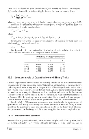
For Example 13.1, the probability distribution of heifer calvings for each sire
across all herds and sexes in all categories are as follows:
Probability in category of response
1 2 3
Sire 1 0.695 0.175 0.131
Sire 2 0.659 0.188 0.153
Sire 3 0.665 0.186 0.149
Sire 4 0.702 0.172 0.126

13.3 Joint Analysis of Quantitative and Binary Traits

Genetic improvement may be based on selecting animals on an index that combines
both quantitative and categorical traits. Optimally, a joint analysis of the quantitative
and categorical traits is required in the prediction of breeding values in such a selec-
tion scheme to adequately account for selection. A linear multivariate model might
be used for such analysis. However, such an analysis suffers from the limitations
associated with the use of a linear model for the analysis of discrete traits mentioned
in Section 13.2. In addition, such a multivariate linear model will not properly
account for the correlated effects of the quantitative traits on the discrete trait.
Foulley et al. (1983) presented a method of analysis to handle the joint analysis of
quantitative and binary traits using a Bayesian approach. It involves fitting a linear
model for the quantitative traits and a non-linear model for the binary trait. This sec-
tion presents this methodology and illustrates its application to an example data set.

13.3.1 Data and model definition

Assume that a quantitative trait, such as birth weight, and a binary trait, such
as calving difficulty (easy versus difficult calving), is being analysed. As in

230 Chapter 13