Page 243 - Linear Models for the Prediction of Animal Breeding Values 3rd Edition

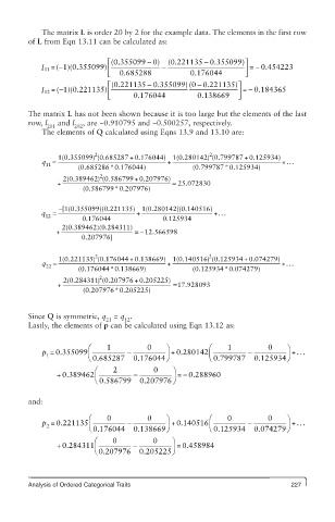
The matrix L is order 20 by 2 for the example data. The elements in the first row
of L from Eqn 13.11 can be calculated as:
−
−
⎡ (0.355099 0) (0.221135 0..355099)⎤
−
l 11 =( 1)(0.355099)− ⎢ ⎣ 0.685288 − 0.176044 ⎥ ⎦ = 0.454223
−
−
−
−
l 12 =( 1)(0.221135) ⎡ ⎢ ⎣ (0.2221135 0.355099) (0 0.221135)⎤ ⎥ ⎦ =0..184365
0.138669
0.176044
The matrix L has not been shown because it is too large but the elements of the last
row, l and l , are −0.910795 and −0.500257, respectively.
201 202
The elements of Q calculated using Eqns 13.9 and 13.10 are:
2
2
1(0.355099) (0.685287 + 0.176044) 1(0.280142) (0.799787 + 0.125934)
q = + +. . .
11
*
*
(0.685286 0.1760444) (0.799787 0.1259344)
2
2(0.389462) (0.586799 + 0.207976)
+ = 25.072830
(0.5867999 0.207976)*
− [1(0.355099)(0.221135) 1(0.280142)(0.140516)
q = + +. . .
12
0.1176044 0.125934
2(0.3894622)(0.284311)
+ = − 12.566598
0.207976]
2
1(0.221135) (00.176044 0.138669) 1(0.140516) (+ 2 0 0.125934 + 0.074279)
q = + +. . .
22
*
(0.176044 0.138669) (0.125934 0.074279)
*
2
2(0.2844311) (0.207976 + 0.205225)
+ = 17.9280093
(0.207976 0.205225)
*
Since Q is symmetric, q = q .
21 12
Lastly, the elements of p can be calculated using Eqn 13.12 as:
æ 1 0 ö æ 1 0 ö
p = 0.355099 ç - ÷ + 0.280142 ç - ÷ + ...
1
è 0.685287 0.176044 ø è 0.7997887 0.125934 ø
æ 2 0 ö
-
+ 0.389462 ç - ÷ = 0.288960
è 0.586799 0 0.207976 ø
and:
æ 0 0 ö æ 0 0 ö
p = 0.221135 ç - ÷ + 0.140516 ç - ÷ + . . .
2
è 0.176044 0.138669 ø è 0.1259334 0.074279 ø
æ 0 0 ö
+ 0.284311 ç - ÷ = 0.458984
è 0.207976 0.2205225 ø

Analysis of Ordered Categorical Traits 227