Page 22 - Feline diagnostic imaging

2.3 Computed Tomography 15

(a) (b)

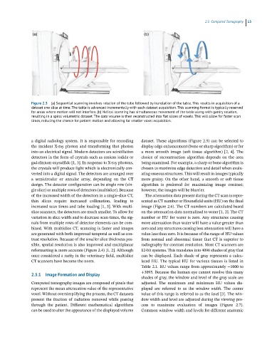
Figure 2.3 (a) Sequential scanning involves rotation of the tube followed by translation of the table. This results in acquisition of a
dataset one slice at time. The table is advanced incrementally with each dataset acquisition. This scanning format is typically reserved
for areas where motion will not interfere. (b) Helical scanning has simultaneous movement of the table along with gantry rotation,
resulting in a spiral volumetric dataset. The data volume is then reconstructed into flat slices of voxels. This will allow for faster scan
times, reducing the chance for patient motion and allowing for smaller voxel acquisition.

a digital radiology system. It is responsible for recording dataset. These algorithms (Figure 2.5) can be selected to
the incident X‐ray photon and transforming that photon display edge enhancement (bone or sharp algorithm) or for
into an electrical signal. Modern detectors are scintillation a more smooth image (soft tissue algorithm) [2, 4]. The
detectors in the form of crystals such as cesium iodide or choice of reconstruction algorithm depends on the area
gadolinium oxysulfide [1, 3]. In response to X‐ray photons, being examined. For example, a sharp or bone algorithm is
the crystals will produce light which is electronically con- chosen to maximize edge detection and detail when evalu-
verted into a digital signal. The detectors are arranged over ating osseous structures. This will result in images typically
a semicircular or annular array, depending on the CT more grainy. On the other hand, a smooth or soft tissue
design. The detector configuration can be single row (sin- algorithm is preferred for maximizing image contrast;
gle slice) or multiple rows of detectors (multislice). Because however, the images will be blurrier.
of the increased width of the detectors in a single‐slice CT, The attenuation data present during the CT scan is repre-
thin slices require increased collimation, leading to sented as CT number or Hounsfield units (HU) on the final
increased scan times and tube loading [1, 3]. With multi- image (Figure 2.6). The CT numbers are calculated based
slice scanners, the detectors are much smaller. To allow for on the attenuation data normalized to water [1, 2]. The CT
variation in slice width and to decrease scan times, the sig- number or HU for water is zero. Any structures causing
nals from multiple rows of detector elements can be com- more attenuation than water will have a value greater than
bined. With multislice CT, scanning is faster and images zero and any structures causing less attenuation will have a
are generated with both improved temporal as well as con- value less than zero. It is because of the range of HU values
trast resolution. Because of the smaller slice thickness pos- from normal and abnormal tissue that CT is superior to
sible, spatial resolution is also improved and multiplanar radiography for contrast resolution. Most CT scanners are
reformatting is more accurate (Figure 2.4) [1, 2]. Although 12‐bit systems. This translates into 4096 shades of gray that
once considered a rarity in the veterinary field, multislice can be displayed. Each shade of gray represents a calcu-
CT scanners have become the norm. lated HU. The typical HU for various tissues is listed in
Table 2.1. HU values range from approximately −1000 to
+3095. Because the human eye cannot resolve this many
2.3.1 Image Formation and Display
shades of gray, the window and level of the gray scale are
Computed tomography images are composed of pixels that adjusted. The maximum and minimum HU values dis-
represent the mean attenuation value of the representative played are referred to as the window width. The center
voxel. Without oversimplifying the process, the CT datasets value of this range is referred to as the level [3]. The win-
present the fraction of radiation removed while passing dow width and level are adjusted during the viewing pro-
through the patient. Different mathematical algorithms cess to maximize evaluation of images (Figure 2.7).
can be used to alter the appearance of the displayed volume Common window width and levels for different anatomic