Page 580 - Microeconomics, Fourth Edition

c13marketstructureandcompetition.qxd 7/30/10 10:44 AM Page 554

554 CHAPTER 13 MARKET STRUCTURE AND COMPETITION

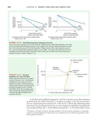
Coca-Cola's price (dollars per unit) $12.50 D 8 Coca-Cola's price (dollars per unit) $13.50 D 12

$7.50
MC
$5.00
MR
MR $5.00 MC
8 12
0 30 50 0 34
Coca-Cola's quantity Coca-Cola's quantity
(million of units per year) (million of units per year)
(a) Coke's profit-maximization problem when (b) Coke's profit-maximization problem when
Pepsi's price = $8 Pepsi's price = $12
FIGURE 13.10 Profit-Maximizing Price Setting by Coca-Cola
MC is Coca-Cola’s marginal cost curve. Panel (a): If Pepsi’s price is $8, Coke’s demand curve is D 8 ,
and its corresponding marginal revenue curve is MR 8 . Coca-Cola will maximize profit at a quan-
tity of 30 units and a price of $12.50. Panel (b): If Pepsi’s price is $12, Coke’s demand curve is
D 12 , and its corresponding marginal revenue curve is MR 12 . Coca-Cola will maximize profit at a
quantity of 34 units and a price of $13.50. These results can be used to plot Coca-Cola’s price
reaction function, shown in Figure 13.11.

R (Coke's reaction
1
function)
P 2 (Pepsi's price, dollars per unit)
Bertrand

prices
R (Pepsi's reaction
FIGURE 13.11 Bertrand $10.14 equilibrium E M Monopoly
$8.26
2
Equilibrium for Coke and Pepsi function)
Coke’s reaction function is R 1 . Pepsi’s
reaction function is R 2 . The Bertrand
equilibrium occurs where the two
reaction functions intersect (point E,
where Coke charges a price of $12.56
and Pepsi charges a price of $8.26).
This differs from the monopoly equi-
librium (point M, where Coke’s price $12.56 $13.80
would be $13.80 and Pepsi’s price P (Coca-Cola's price, dollars per unit)
1
would be $10.14).
At the Bertrand equilibrium (point E ), each firm chooses a price that maximizes
its profit given the other firm’s price. 31 As shown in Figure 13.11, this occurs where
the two reaction functions intersect (P* $12.56, P* $8.26). By substituting these
1
2
prices back into the demand functions, we can compute the equilibrium quantities for
Coca-Cola and Pepsi: Q* 30.28 million units and Q* 21.26 million units. In fact,
1
2
31 You will see in Chapter 14 that the Bertrand equilibrium, like the Cournot equilibrium, is a particular
example of a Nash equilibrium. For this reason, some textbooks refer to the Bertrand equilibrium as the
Nash equilibrium in prices.