Page 581 - Microeconomics, Fourth Edition

c13marketstructureandcompetition.qxd 7/30/10 10:44 AM Page 555

13.4 OLIGOPOLY WITH HORIZONTALLY DIFFERENTIATED PRODUCTS 555
the average (inflation-adjusted) prices over the time period of GVL’s study
(1968–1986) were actually $12.96 for Coca-Cola and $8.16 for Pepsi. The correspon-
ding quantities were 30.22 million units and 22.72 million units. Thus, the Bertrand
model, when applied to the demand curves estimated by GVL, does a good job of
matching the actual pricing behavior of these two firms in the U.S. market.
Pepsi’s equilibrium price is so much lower than Coca-Cola’s price for two impor-
tant reasons. First, Pepsi’s marginal cost is lower than Coke’s. Second, and more subtly,
Pepsi’s own price elasticity of demand is larger than Coke’s (as shown in Table 2.7). 32
Since we know (from Chapter 11) that profit maximization along a downward-sloping
demand curve implies an inverse elasticity pricing rule (IEPR), applying the IEPR to
Coke and Pepsi’s pricing problem implies that Pepsi should have a smaller markup than
Coke. A smaller markup applied to a smaller marginal cost makes Pepsi’s price lower
than Coca-Cola’s.
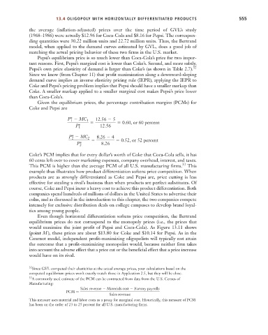
Given the equilibrium prices, the percentage contribution margins (PCMs) for
Coke and Pepsi are
P* MC 1 12.56 5
1
0.60, or 60 percent
P* 1 12.56
P* MC 2 8.26 4
2
0.52, or 52 percent
P* 2 8.26
Coke’s PCM implies that for every dollar’s worth of Coke that Coca-Cola sells, it has
60 cents left over to cover marketing expenses, company overhead, interest, and taxes.
This PCM is higher than the average PCM of all U.S. manufacturing firms. 33 This
example thus illustrates how product differentiation softens price competition. When
products are as strongly differentiated as Coke and Pepsi are, price cutting is less
effective for stealing a rival’s business than when products are perfect substitutes. Of
course, Coke and Pepsi incur a heavy cost to achieve this product differentiation. Both
companies spend hundreds of millions of dollars in the United States to advertise their
colas, and as discussed in the introduction to this chapter, the two companies compete
intensely for exclusive distribution deals on college campuses to develop brand loyal-
ties among young people.
Even though horizontal differentiation softens price competition, the Bertrand
equilibrium prices do not correspond to the monopoly prices (i.e., the prices that
would maximize the joint profit of Pepsi and Coca-Cola). As Figure 13.11 shows
(point M ), these prices are about $13.80 for Coke and $10.14 for Pepsi. As in the
Cournot model, independent profit-maximizing oligopolists will typically not attain
the outcome that a profit-maximizing monopolist would, because neither firm takes
into account the adverse effect that a price cut or the beneficial effect that a price increase
would have on its rival.

32 Since GVL computed their elasticities at the actual average prices, your calculations based on the
computed equilibrium prices won’t exactly match those in Application 2.5, but they will be close.
33 A commonly used estimate of the PCM can be contructed from data from the U.S. Census of
Manufacturing:
Sales revenue Materials cost Factory payrolls
PCM
Sales revenue
This measure uses material and labor costs as a proxy for marginal cost. Historically, this measure of PCM
has been on the order of 23 to 25 percent for all U.S. manufacturing firms.