Page 339 - Economics

CONFIRMING PAGES

CHAPTER 15
291
Extending the Analysis of Aggregate Supply
The Phillips Curve FIGURE 15.7 The short-run effect of changes in
We can demonstrate the short-run tradeoff between the rate aggregate demand on real output and the price
level. Comparing the effects of various possible increases in
of inflation and the rate of unemployment aggregate demand leads to the conclusion that the larger the increase
through the Phillips Curve , named after in aggregate demand, the higher the rate of inflation and the greater
the increase in real output. Because real output and the unemployment
A. W. Phillips, who developed the idea in rate move in opposite directions, we can generalize that, given short-
Great Britain. This curve, generalized in run aggregate supply, high rates of inflation should be accompanied by
Figure 15.6a , suggests an inverse relationship low rates of unemployment.
between the rate of inflation and the rate of
O 15.1 AS
unemployment. Lower unemployment rates
Phillips Curve
(measured as leftward movements on the P 3
horizontal axis) are associated with higher rates of inflation
(measured as upward movements on the vertical axis). P 2 AD 3
The underlying rationale of the Phillips Curve be- Price level
comes apparent when we view the short-run aggregate P 1
supply curve in Figure 15.7 and perform a simple mental P 0
AD 2
experiment. Suppose that in some short-run period aggre-
to AD , either because
gate demand expands from AD 0 2 AD 0
firms decided to buy more capital goods or the govern- AD 1
ment decided to increase its expenditures. Whatever the 0 Q 0 Q 1 Q 2 Q 3
cause, in the short run the price level rises from P to P Real domestic output
2
0
and real output rises from Q to Q . A decline in the un-
2
0
employment rate accompanies the increase in real output. inflation and the growth of real output would have been
Now let’s compare what would have happened if the smaller (and the unemployment rate higher).
increase in aggregate demand had been larger, say, from The generalization we draw from this mental experi-
AD to AD . The new equilibrium tells us that the amount ment is this: Assuming a constant short-run aggregate
0
3
of inflation and the growth of real output would both have supply curve, high rates of inflation are accompanied by
been greater (and that the unemployment rate would have low rates of unemployment, and low rates of inflation are
been lower). Similarly, suppose aggregate demand during accompanied by high rates of unemployment. Other things
the year had increased only modestly, from AD to AD . equal, the expected relationship should look something
0
1
Compared with our shift from AD to AD , the amount of like Figure 15.6a.
0
2
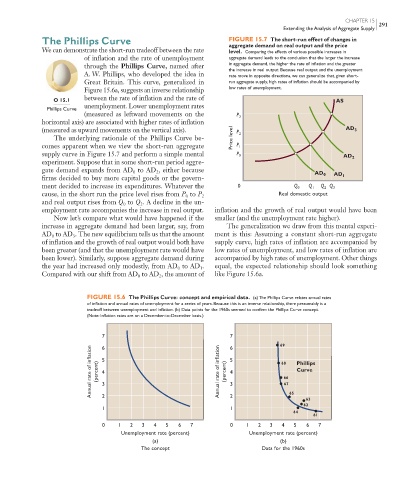
FIGURE 15.6 The Phillips Curve: concept and empirical data. (a) The Phillips Curve relates annual rates
of inflation and annual rates of unemployment for a series of years. Because this is an inverse relationship, there presumably is a
tradeoff between unemployment and inflation. (b) Data points for the 1960s seemed to confirm the Phillips Curve concept.
(Note: Inflation rates are on a December-to-December basis.)

7 7
69
Annual rate of inflation (percent) 5 4 3 Annual rate of inflation (percent) 5 4 3 68 66 Phillips
6
6
Curve
67
65
2
2
63
62
1 1
64
61
0 1 2 3 4 5 6 7 0 1 2 3 4 5 6 7
Unemployment rate (percent) Unemployment rate (percent)
(a) (b)
The concept Data for the 1960s

mcc26632_ch15_284-301.indd 291 9/1/06 3:17:10 PM
9/1/06 3:17:10 PM
mcc26632_ch15_284-301.indd 291