Page 161 - Fiber Optic Communications Fund

142 Fiber Optic Communications

∗
∗
same as that of having a a =−1. Therefore, the ensemble average of a a is zero when k ≠ l. When k = l,
l k l k
∗ 2
< a a >=< |a | >= 1. (4.11)
l k k
The terms in Eq. (4.9) can be divided into two groups; terms with k = l and terms with k ≠ l,
[ ]
L
L ∑ ∑
L
∑
∗
2
2
2
(f)= A |̃p(f)| lim 1 < |a | > + < a a > e i2f(l−k)T b . (4.12)
m 0 k l k
L→∞ (2L + 1)T
b k=−L l=−L k=−L,k≠l
Using Eqs. (4.10) and (4.11) in Eq. (4.12), we find
2 2
2L + 1 A |̃p(f)|
0
2
2
(f)= A |̃p(f)| lim = . (4.13)
m 0 L→∞ (2L + 1)T
b T b
4.4.1 Polar Signals
Consider a polar signal with RZ pulses. The pulse shape function p(t) is
( )
t
p(t)= rect , (4.14)
xT b
̃ p(f)= xT sinc (xT f), (4.15)
b
b
where sinc (y)= sin (y)∕(y). Using Eq. (4.15) in Eq. (4.13), we find
2 2
RZ
2
(f)= A x T sinc (xT f). (4.16)
m 0 b b
When x = 1, this corresponds to a NRZ pulse and the PSD is
NRZ 2 2
(f)= A T sinc (T f). (4.17)
m 0 b b
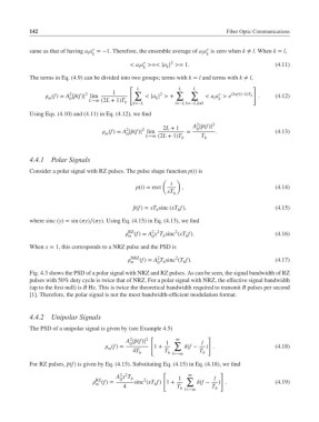
Fig. 4.3 shows the PSD of a polar signal with NRZ and RZ pulses. As can be seen, the signal bandwidth of RZ
pulses with 50% duty cycle is twice that of NRZ. For a polar signal with NRZ, the effective signal bandwidth
(up to the first null) is B Hz. This is twice the theoretical bandwidth required to transmit B pulses per second
[1]. Therefore, the polar signal is not the most bandwidth-efficient modulation format.

4.4.2 Unipolar Signals
The PSD of a unipolar signal is given by (see Example 4.5)

[ ]
2 2 ∞
A |̃p(f)| 1 ∑ l
0
(f)= 1 + (f − ) . (4.18)
m
4T T T
b b l=−∞ b
For RZ pulses, ̃p(f) is given by Eq. (4.15). Substituting Eq. (4.15) in Eq. (4.18), we find
[ ∞ ]
2 2
A x T b 1 ∑ l
0
RZ
2
(f)= sinc (xT f) 1 + (f − ) . (4.19)
m b
4 T T
b l=−∞ b