Page 229 - Six Sigma Advanced Tools for Black Belts and Master Black Belts

August 31, 2006
Char Count= 0
3:4
JWBK119-14
214 Data Transformation for Geometrically Distributed Quality Characteristics
14.3.1 Quesenberry’s Q transformation
5
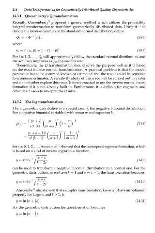
Recently, Quesenberry proposed a general method which utilizes the probability
integral transformation to transform geometrically distributed data. Using −1 to
denote the inverse function of the standard normal distribution, define
−1
Q i =− (u i ) , (14.6)
where
u i = F (x i ; p) = 1 − (1 − p) . (14.7)
x i
For i = 1, 2, ... , Q i will approximately follow the standard normal distribution, and
the accuracy improves as p 0 approaches zero.
Theoretically, the Q transformation should serve the purpose well as it is based
on the exact inverse normal transformation. A practical problem is that the model
parameter has to be assumed known or estimated and the result could be sensitive
to erroneous estimates. A sensitivity study of this issue will be carried out in a later
section to further explore this issue. It is not practical to use the inverse normal trans-
formation if it is not already built in. Furthermore, it is difficult for engineers and
other chart users to interpret the results.

14.3.2 The log transformation
The a geometric distribution is a special case of the negative binomial distribution.
For a negative binomial variable v with mean m and exponent k,

(v + k) m v m −k

p(v) = 1 + (14.8)
v! (k) m + k k
v
(v + k − 1)! m k k
=
v! (k − 1)! m + k m + k
14
for v = 0, 1, 2, ... . Anscombe showed that the corresponding transformation, which
is based on a kind of inverse hyperbolic function,

v + c
−1
y = sinh , (14.9)
k − 2c
can be used to transform a negative binomial distribution to a normal one. For the
geometric distribution, as we have k = 1 and v = x − 1, the transformation becomes

v + c
−1
y = sinh . (14.10)
1 − 2c
14
Anscombe also showed that a simpler transformation, known to have an optimum
property for large m and k ≥ 1, is
1
y = ln v + k . (14.11)
2
For the geometric distribution the transformation becomes
1

y = ln x − .
2