Page 230 - Six Sigma Advanced Tools for Black Belts and Master Black Belts

3:4
August 31, 2006
Char Count= 0
JWBK119-14
Some Possible Transformations 215
In fact, when x is large, which is, for example, the case when a high-quality process
is monitored based on cumulative counts of conforming items between two noncon-
forming ones, both the inverse hyperbolic and the log transformation are equivalent
to the simple logarithmic transformation. This is because

−1
2
sinh x = ln x + x + 1
≈ ln (x + x) = ln 2 + ln x. (14.12)
As will be seen later, the log transformation, although it can be used, is not very good
for geometrically distributed quantities.

14.3.3 A double square root transformation
The method that we propose to transform a geometrically distributed quantity into a
normal one is through the use of the double square root transformation
y = x 1/4 , x ≥ 0. (14.13)
The background behind using the double square root transformation is as follows.
It is well known that the square root transformation can be used to convert positively
skewed quantities to normal. However, the geometric distribution is highly skewed,
and it will be observed that after the square root transformation it is still positively
skewed. In fact, we should use x 1/r for some r > 2. However, considering the accu-
racy and simplicity, the double square root transformation is preferred as it can be
performed using some simple spreadsheet software or even a simple calculator.
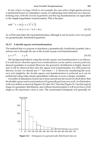
Anumberofsimulationstudieshavebeencarriedout,theresultsofwhichshowthat
thedoublesquareroottransformationwillgenerallyperformverywell.Anillustration
with a set of data is shown in Figures 14.1 and 14.2. Note that Figure 14.1 has the typical
shape of a geometric distribution, and without transformation it will never have a bell
shape as the maximum value is zero. The transformed histogram will generally be

Raw Data

300

200

100

0
0 50 100 150 200 250 300 350 400 450 500 550 600 650 700

Figure 14.1 Histogram of a geometrically distributed data set.