Page 234 - Six Sigma Advanced Tools for Black Belts and Master Black Belts

August 31, 2006
3:4
JWBK119-14
Char Count= 0
Sensitivity Analysis of the Q Transformation 219
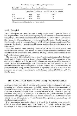
Table 14.4 Comparison of three transformations.
Skewness Kurtosis Anderson--Darling statistic
X 1/4 0.12* 2.27 0.90*
ln X −0.35 2.61* 1.0
Q-transformation −0.22 2.35 1.0
*Closest to a normal distribution on a given statistic.

14.4.2 Example 2
The double square root transformation is easily implemented in practice. In one of
our projects with a local manufacturing company the problem of nonnormality was
brought up. The double square root transformation has proved to be very useful.
Here an actual data set of particle counts is used for illustration. The histogram has
the shape of a negative exponential curve, which is the continuous counterpart of the
geometric distribution. Hence the double square root transformation is thought to be
appropriate.
Table 14.4 presents some normality test statistics for the data set when the three
transformations are used. The double square root transformation is seen to be most
suitable in terms of skewness and Anderson--Darling statistic, while for kurtosis the
log transformation is preferable.
The purpose of this application was to transform the data to normal so that tradi-
tional control charts together with run rules could be used. The comparison of the
original control chart and the one produced after adopting the double square root
transformation is shown in Figure 14.4. It is clear that the transformed chart is more
suitable in this case. It should be pointed out that a simple test of normality must be
performed before using any transformation in a practical situation. Only when the
normality test is accepted can run rules and techniques such as EWMA and CUSUM
then be used.

14.5 SENSITIVITY ANALYSIS OF THE Q TRANSFORMATION

As discussed previously, the Q transformation should be the most appropriate trans-
formation as it is based on the exact probability values. However, the parameter of
the distribution is assumed known and it would be interesting to see how the Q trans-
formation is affected by errors in the value of p. Recall that the Q statistic is given by
equations (14.6) and (14.7). When p = p 0 is constant, the Q transformation can give
independent and approximately standard normal statistics. Note that because of the
discrete nature of the data the approximate normality depends on p 0 ; a smaller p 0 will
give better approximations.
If an incorrect or inaccurate value of p 0 is used, the Q statistic could be totally
different from what it should have been. Changes in Q statistic can be studied based
on changes in p 0 . This will be illustrated as follows with a numerical example.