Page 255 - Six Sigma Advanced Tools for Black Belts and Master Black Belts

OTE/SPH
OTE/SPH
3:5
Char Count= 0
August 31, 2006
JWBK119-16
240 A Glossary for Design of Experiments with Examples
Response Response

−1 0 +1 −1 0 +1
Factor Level Factor Level
k
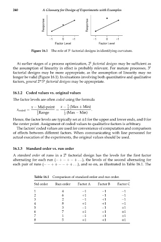
Figure 16.1 The role of 3 factorial designs in identifying curvature.

k
At earlier stages of a process optimization, 2 factorial designs may be sufficient as
the assumption of linearity in effect is probably relevant. For mature processes, 3 k
factorial designs may be more appropriate, as the assumption of linearity may no
longer be valid (Figure 16.1). In situations involving both quantitative and qualitative
m n
factors, general 2 3 factorial designs may be appropriate.
16.1.2 Coded values vs. original values

The factor levels are often coded using the formula
1
x − Mid-point x − (Max + Min)
2
x coded = = .
1 Range 1 (Max − Min)
2 2
Hence, the factor levels are typically set at ±1 for the upper and lower ends, and 0 for
the center point. Assignment of coded values to qualitative factors is arbitrary.
The factors’coded values are used for convenience of computation and comparison
of effects between different factors. When communicating with line personnel for
actual execution of the experiments, the original values should be used.

16.1.3 Standard order vs. run order
k
A standard order of runs in a 2 factorial design has the levels for the first factor
alternating for each run (−+−+−+ ...), the levels of the second alternating for
each pair of runs (−−++−−++ ...), and so on, as illustrated in Table 16.1. The

Table 16.1 Comparison of standard order and run order.
Std order Run order Factor A Factor B Factor C

1 4 −1 −1 −1
2 6 +1 −1 −1
3 2 −1 +1 −1
4 8 +1 +1 −1
5 3 −1 −1 +1
6 7 +1 −1 +1
7 1 −1 +1 +1
8 5 +1 +1 +1