Page 258 - Six Sigma Advanced Tools for Black Belts and Master Black Belts

OTE/SPH
OTE/SPH
August 31, 2006
3:5
JWBK119-16
Char Count= 0
Residual Analysis 243
and its adjusted counterpart
R 2 = 1 − SS Error /ν Error .
adj
SS Total /(N − 1)
2
For comparison of models, use R : the higher the value, the better the model. To
adj
2
check the adequacy of the ‘best’ model, use R . This metric estimates the proportion
of observed variation accounted for by the model selected. For practical purposes,
2
choose a parsimonious model with sufficient R .

16.3 RESIDUAL ANALYSIS

From the ANOVA table in Table 16.2, it may be observed that the significance of a main
effect or interaction is dependent on MS Error . Hence, it is important that we examine
the distribution of the residuals. Under ANOVA, the residuals are assumed to be
normally and independently distributed about a null mean and constant variance:
2
ε ∼ NID(μ = 0, σ = constant). We will examine some of the consequences when
these assumptions are violated.

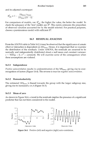
16.3.1 Independence

Positive autocorrelation results in underestimation of the MS Error , giving rise to over-
recognition of factors (Figure 16.4). The reverse is true for negative autocorrelation.

16.3.2 Homoskedasticity
The estimated MS Error is biased towards the group with the larger subgroup size,
giving rise to increased α or β (Figure 16.5).

16.3.3 Mean of zero
As shown in Figure 16.6, a trend in the residuals implies the presence of a significant
predictor that has not been considered in the model.

1.5 1.5
1 0.5 1
0.5
Residuals −0.5 0 0 5 10 15 20 Residuals −0.5 0 0 5 10 15 20

−1 −1
−1.5 −1.5
Observation Order Observation Order
Figure 16.4 Positive (left) and negative (right) auto-correlation.