Page 262 - Six Sigma Advanced Tools for Black Belts and Master Black Belts

OTE/SPH
OTE/SPH
August 31, 2006
3:5
Char Count= 0
JWBK119-16
Fractional Factorial Designs 247
Table 16.5 Overview of fractional factorial design when only main effects and two-way
interactions are of interest.
k
Factors 2 design Required runs 2 k−p design Delta
2
2
2 2 = 4 3 2 = 4
3
3 2 3 = 8 6 2 = 8
4
4 2 4 = 16 10 2 = 16
4
5 2 5 = 32 15 2 = 16 16 (50.00 %)
5
6 2 6 = 64 21 2 = 32 32 (50.00 %)
5
7 2 7 = 128 28 2 = 32 96 (75.00 %)
6
8 2 8 = 256 36 2 = 64 192 (75.00 %)
6
9 2 9 = 512 45 2 = 64 448 (87.50 %)
6
10 2 10 = 1024 55 2 = 64 960 (93.75 %)
16.5.1 Confounding and aliasing
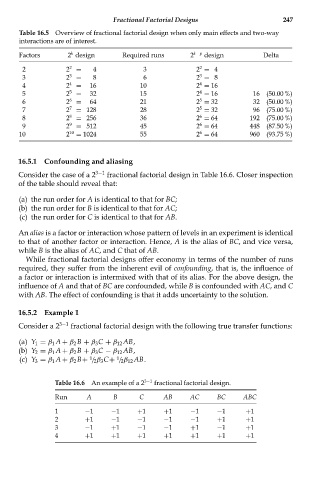
Consider the case of a 2 3−1 fractional factorial design in Table 16.6. Closer inspection
of the table should reveal that:
(a) the run order for A is identical to that for BC;
(b) the run order for B is identical to that for AC;
(c) the run order for C is identical to that for AB.

An alias is a factor or interaction whose pattern of levels in an experiment is identical
to that of another factor or interaction. Hence, A is the alias of BC, and vice versa,
while B is the alias of AC, and C that of AB.
While fractional factorial designs offer economy in terms of the number of runs
required, they suffer from the inherent evil of confounding, that is, the influence of
a factor or interaction is intermixed with that of its alias. For the above design, the
influence of A and that of BC are confounded, while B is confounded with AC, and C
with AB. The effect of confounding is that it adds uncertainty to the solution.

16.5.2 Example 1
Consider a 2 3−1 fractional factorial design with the following true transfer functions:

(a) Y 1 = β 1 A+ β 2 B + β 3 C + β 12 AB,
(b) Y 2 = β 1 A+ β 2 B + β 3 C − β 12 AB,
(c) Y 3 = β 1 A+ β 2 B+ / 2β 3 C+ / 2β 12 AB.
1
1
Table 16.6 An example of a 2 3−1 fractional factorial design.
Run A B C AB AC BC ABC

1 −1 −1 +1 +1 −1 −1 +1
2 +1 −1 −1 −1 −1 +1 +1
3 −1 +1 −1 −1 +1 −1 +1
4 +1 +1 +1 +1 +1 +1 +1