Page 257 - Maxwell House

Chapter 5 237

describing the power radiated by the electric and magnetic radiator. In both cases, the
enlarging the electrical dimensions, i.e. their effective aperture (see Section 5.2.11 of this
chapter) of element escalates its radiating power and directivity. Therefore, we can assume that
an assembly of radiating elements in a proper electrical and geometrical configuration called
antenna array is the solution. The individual elements may be of any type (wire dipoles,
loops, Huygens’, or their combination put in the same spot). Usually, all array elements are
identical. This is not necessary, but it is practical and simpler for design and fabrication. If so,
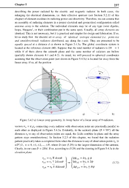
let us study first the discrete set or array of identical isotropic elemental (i.e. point-size
and omnidirectional) radiators distributed, say along the z-axis. They are presumed to be
equally spaced at a distance d as shown in Figure 5.4.3a. The global coordinate system is
located at the reference element (#0). Suppose that the total number of radiators is 2 + 1
while N of them above the azimuth plane and the same number of radiators are bellow
(partially shown elements #-1 and #-2). As usual, we will proceed in spherical coordinates
assuming that the observation point (not shown in Figure 5.4.3a) is located far away from the
linear array. If so, all the position

N

3
2
d
1
d 3
0
-1
-2

a) b)

Figure 5.4.3 a) Linear array geometry, b) Array factor of a linear array of 9 radiators.
vectors = connecting every radiator with observation point are practically parallel to
0

each other as displayed in Figure 5.4.3a. Evidently, in the azimuth plane ( = 90°) all the
distances to any of observation points are equal, the fields combine in phase and the array

pattern stays omnidirectional. In Section 5.2.5 of this chapter, we found that the radiation
pattern practically takes a completed form when the distances to any of observation points ≫

⁄ , = 0, ±1, ±2, … , ±, where D (see (5.29)) is the largest dimension of the antenna.
2

Clearly, in our case = 2. If so, according to (5.29) and the drawing in Figure 5.4.3a in the
elevation plane
±1 = ∓ cos ∆ ±1 = ±
0
0
= ∓ 2cos ∆ = ± 2
±2 0 � ⇒ � ±2 0 (5.72)
… …
± = ∓ cos ∆ ± = ±
0
0