Page 259 - Maxwell House

Chapter 5 239

1 −
= ∫ () (5.75)

2 −
Here the array factor () must be defined over the whole interval || ≤ . The reader
probably noticed in (5.73) and (5.75) the far-
reaching analogy between a signal waveform
and its spectrum (1.82) in Chapter 1. It means,
for example, that the integral in (5.75) can be
z-axis, evaluated numerically using Fast Fourier
Transform (FFT) [38] the same way as in signal
processing. Consider the trivial synthesis
example. Suppose that a customer requested an
antenna with the sector pattern shown in Figure
Figure 5.4.4a Desired sector pattern 5.4.4a to minimize the spillover loss in the dish
antenna illustrated in figure 5.2.13. It means, for
example, that for 2 = 60°
0
1, if 60° < < 120°
() = � (5.76)
0, if elsewhere
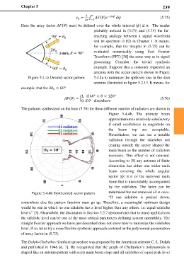
The patterns synthesized on the base (5.76) for three different number of radiators are shown in
Figure 5.4.4b. The primary beam
approximation is relatively satisfactory
if small oscillations in magnitude on
the beam top are acceptable.
Nevertheless, we can see a notable
radiation through the sidelobes not
ceasing outside the sector shaped the
main beam as the number of radiators
increases. This effect is not unusual.
According to [5] any antenna of finite
dimension has either one wider main
beam covering the whole angular
sector || ≤ or the narrower main
beam that is unavoidably accompanied
by the sidelobes. The latter can be
Figure 5.4.4b Synthesized sector pattern minimized but not removed all at once.
“If one sidelobe is pushed down,
somewhere else the pattern function must go up. Therefore, a meaningful optimum design
would be one in which no one sidelobe has a level higher than any others, i.e. equal sidelobe
levels.” [5]. Meanwhile, the discussion in Section 5.2.7 demonstrates that in many applications
the sidelobe level can be one of the most critical parameters defining system operability. The
straight Fourier approach we have just described does not show how to minimize the sidelobes
level. If so, let us try a more flexible synthesis approach centered on the polynomial presentation
of array factor in (5.73).

The Dolph-Chebyshev Synthesis procedure was proposed by the American scientist C. L. Dolph
and published in 1946 [6, 7]. He recognized that the graph of Chebyshev’s polynomials is
shaped like an antenna pattern with steep main beam slope and all sidelobes of equal peak level