Page 262 - Maxwell House

242 ANTENNA BASICS

together and displayed by the set of green points. Note that the adjacent radiator separation d
between the even array elements corresponds to the actual distance in wavelength.

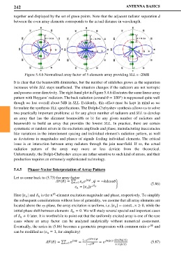
Figure 5.4.6 Normalized array factor of 5 elements array providing SLL = -20dB

It is clear that the beamwidth diminishes, but the number of sidelobes grows as the separation
increases while SLL stays unaffected. The situation changes if the radiators are not isotropic
and possess some directivity. The right-hand plot in Figure 5.4.6 illustrates the same linear array
pattern with Huygens’ radiators. The back radiation (around = 180°) is suppressed quite well
though we lost overall about 5dB in SLL. Evidently, this effect must be kept in mind as we
formulate the synthesis SLL specifications. The Dolph-Chebyshev synthesis allows us to solve
two practically important problems: a) for any given number of radiators and SLL to develop
an array that has the slimmest beamwidth or b) for any given number of radiators and
beamwidth to build an array that provides the lowest SLL. In practice, there are certain
systematic or random errors in the excitation amplitude and phase, manufacturing inaccuracies
like variations in the interelement spacing and individual element's radiation pattern, as well
as deviations in magnitudes and phases of signals feeding individual elements. The critical
issue is an interaction between array radiators through the join near-field. If so, the actual
radiation pattern of the array may more or less deviate from the theoretical.
Unfortunately, the Dolph-Chebyshev arrays are rather sensitive to such kind of errors, and their
production requires an extremely sophisticated technology.

5.4.5 Phasor-Vector Interpretation of Array Pattern
Let us come back to (5.73) for array factor
() = ∑ , = −cos � (5.86)

=0
= | |

Here | | and is the -element excitation magnitude and phase, respectively. To simplify
ℎ

the subsequent considerations without loss of generality, we assume that all array elements are
located above the xy-plane, the array excitation is uniform, i.e. | | = const. , ≥ 0, while the

initial phase shift between elements = 0. We will study several special and important cases

of ≠ 0 later. It is worthwhile to point out that the uniformly excited array is one of the rare

cases where an array factor can be analyzed analytically without numerical assessment.
Eventually, the series in (5.86) becomes a geometric progression with common ratio and

can be modified as ( = 1, for simplicity)

(+1)
1− sin (/2)
() = ∑ = = /2 (5.87)
=0
⁄
1− sin ( 2)