Page 260 - Maxwell House

240 ANTENNA BASICS

relative to the main beam peak (see Figure 5.4.5). We proceed in several simple steps giving
the reader the sense of understanding without serious mathematics.

First, we need to build a bridge
between the antenna factor () and
Chebyshev’s polynomials. To simplify
the subsequent considerations, assume
that the linear array shown in Figure
5.4.3a is exited symmetrically meaning
that − = . Then according to (5.73)

() = + ∑ ( +

0
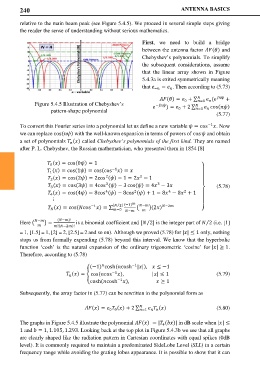
Figure 5.4.5 Illustration of Chebyshev’s − =1 cos()
pattern-shape polynomial ) = + 2 ∑ =1
0
(5.77)
To convert this Fourier series into a polynomial let us define a new variable = cos −1 . Now
we can replace cos() with the well-known expansion in terms of powers of cos and obtain
a set of polynomials () called Chebyshev’s polynomials of the first kind. They are named

after P. L. Chebyshev, the Russian mathematician, who presented them in 1854 [8]

() = cos(0) = 1 ⎫
0
−1
() = cos(1) = cos(cos ) = ⎪
1
2
2
() = cos(2) = 2cos () − 1 = 2 − 1 ⎪
2
3
3
() = cos(3) = 4cos () − 3 cos() = 4 − 3 (5.78)
3
4
4
2
2
() = cos(4) = 8cos () − 8cos () + 1 = 8 − 8 + 1 ⎬
4
⋮ ⎪
⎪
⁄
−1
() = cos(cos ) = ∑ [ 2] (−1) � − �(2) −2
=0 ⎭
−
− (−)!
⁄
⁄
Here � � = is a binomial coefficient and [ 2] is the integer part of 2 (i.e. [1]
!(−2)!
= 1, [1.5] = 1, [2] = 2, [2.5] = 2 and so on). Although we proved (5.78) for || ≤ 1 only, nothing
stops us from formally expending (5.78) beyond this interval. We know that the hyperbolic
function ‘cosh’ is the natural expansion of the ordinary trigonometric ‘cosine’ for || ≥ 1.
Therefore, according to (5.78)

−1
(−1) cosh(cosh ||), ≤ −1
−1
() = �cos(cos ), || ≤ 1 (5.79)

−1
cosh(cosh ), ≥ 1
Subsequently, the array factor in (5.77) can be rewritten in the polynomial form as
() = () + 2 ∑ () (5.80)
0 0

=1
The graphs in Figure 5.4.5 illustrate the polynomial () = | ()| in dB scale when || ≤
4
1 and = 1, 1.105, 1.293. Looking back at the top plot in Figure 5.4.3b we see that all graphs
are clearly shaped like the radiation pattern in Cartesian coordinates with equal spikes (0dB
level). It is commonly required to maintain a predominated SideLobe Level (SLL) in a certain
frequency range while avoiding the grating lobes appearance. It is possible to show that it can