Page 282 - Maxwell House

262 ANTENNA BASICS

26
depicted in Figure 5.6.1b . The probable 3D pattern in dB scale is also presented and displays
the array directivity in both planes (pencil beam). It is standard practice to assume that all
radiators are uniformly spread in the XY-plane as shown in Figure 5.6.1a and to run far field
analysis in spherical coordinates (see Figure 5.6.1b). In line with this drawing, the element (0,
0) is located at the origin while the element (, ) is shifted into position ( , ). As shown

earlier, the phase shift between waves radiated by these elements in far field region is
proportional to the inter-element separation, which is ( , ), and angular positions (, )

of the observation point P. According to (5.29) and Figure 5.6.1b, it yields

= −( sin cos + sin sin) (5.104)

If so, the total electric field emitted by the whole planar array is the ordinary double sum
(, ) = ∑ ∑ (5.105)
=0
Σ
=0
Here = | | is the far field magnitude (complex in general) radiated by the element
th
located at a cross point of the “m ” row with “n ” column. To further illustrate the planar array
th
characteristics suppose that = and = + . Such an element excitation

method is typical in practical applications. The expression (5.105) can be rewritten as a product
(, ) = ∑ | | − sin cos− ∑ | | − sin sin− (5.106)
=0

Σ
=0
Evidently, each sum-factor in (5.106) represents the linear array, and the whole expression
follows the pattern multiplication rule (5.74)
(, ) = (, ) ∙ (, ) ∙ (, ) (5.107)

Here (, ) and (, ) is the first and second sum-factor in (5.106), respectively.

The additional factor (, ) reflects the influence of array element self-directivity. Both sum-
factors can be expressed in simple closed form if the amplitude excitation of the entire array is
uniform and phase distribution is progressive, i.e. | |= | | = 1, = − , =

1

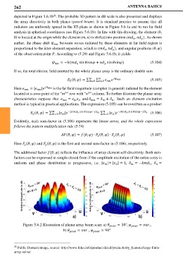
Figure 5.6.2 Illustration of planar array beam scan: a) = 30°, = .,
b) = . , = 90°

26 Public Domain Image, source: http://www.feko.info/product-detail/productivity_features/large-finite-
array-solver