Page 283 - Maxwell House

Chapter 5 263

− where the constants are defined the line lengths inside the TTD units (see Figure
2 1,2
5.5.5). Then according to (5.32) in uv-coordinates, i.e. = sin cos and = sin sin,

sin�(+1) (− )/2� sin�(+1) (− )/2� ⎫
(, ) = () ∙ ∙ (+1)sin ( (− )/2) ⎪
(+1)sin ( (− )/2) (5.108)
= sin cos = / ⎬
1

= sin sin = / ⎪
2
⎭
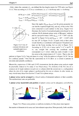
Since the angles ( , ) are the given parameter we
can find the required length and of line in the TTD
1
2
units connected to each radiator in the array. Figure 5.6.2
illustrates the family of normalized pattern developed by the
uniform 10x10 elements planar array of Huygens’ radiators
and its scan performance while = 0° − 300° with the
step 60° in Figure 5.6.2a and = −60° − (+60°) with
the step 20° in Figure 5.6.2b. A quick look at these plots
reveals that the uv-coordinates well represent 3D patterns and
Figure 5.6.3 Line of map out the beam steering. Let us refer to Figure 5.6.3.
constant elevation and According to (5.32) / = tan and + = sin . If
2
2
2
azimuth angle in uv- so, any straight line crossing the coordinate origin
coordinates corresponds to = . while any circle of radii < 1 and
the center at the origin relates to = . That is why the
patterns in Figure 5.6.2a “sing and dance in a ring” while the patterns in Figure 5.6.2b “line up
for a military parade.” Note that the expressions in (5.33) allow us to return to patterns in
elevation and azimuth coordinates.

Meanwhile, expressions (5.106) and (5.107) demonstrate that the planar array analysis might
be practically reduced to the study of two linear arrays. The elements of the first one are a
common set of single radiators in each row or column while the second one is a configuration
where the role of the single radiator is performed by this row or column. In other words, we
may extend many ideas from Section 5.5 and 5.6 to planar arrays.

A planar array can be arranged in a broad variety of elemental radiators or their assembly.
The unidirectional ones are preferable.
A planar array beamwidth and position of pattern zeroes can be adequately controlled by

SLL = -13dB SLL = -23dB
SLL = -13dB

a) b)

Figure 5.6.4 Planar array pattern: a) uniform excitation, b) One plane sinus-tapered

the number of elements in the array and inter-element separation. More precisely, both variables