Page 651 - Krugmans Economics for AP Text Book_Neat

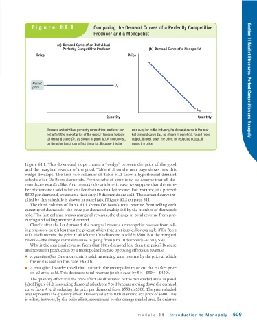
figure 61.1 Comparing the Demand Curves of a Perfectly Competitive
Producer and a Monopolist

(a) Demand Curve of an Individual
Perfectly Competitive Producer (b) Demand Curve of a Monopolist
Price Price

Market D Section 11 Market Structures: Perfect Competition and Monopoly
price C

D M
Quantity Quantity

Because an individual perfectly competitive producer can- sole supplier in the industry, its demand curve is the mar-
not affect the market price of the good, it faces a horizon- ket demand curve D M , as shown in panel (b). To sell more
tal demand curve D C , as shown in panel (a). A monopolist, output, it must lower the price; by reducing output, it
on the other hand, can affect the price. Because it is the raises the price.

Figure 61.1. This downward slope creates a “wedge” between the price of the good
and the marginal revenue of the good. Table 61.1 on the next page shows how this
wedge develops. The first two columns of Table 61.1 show a hypothetical demand
schedule for De Beers diamonds. For the sake of simplicity, we assume that all dia-
monds are exactly alike. And to make the arithmetic easy, we suppose that the num-
ber of diamonds sold is far smaller than is actually the case. For instance, at a price of
$500 per diamond, we assume that only 10 diamonds are sold. The demand curve im-
plied by this schedule is shown in panel (a) of Figure 61.2 on page 611.
The third column of Table 61.1 shows De Beers’s total revenue from selling each
quantity of diamonds—the price per diamond multiplied by the number of diamonds
sold. The last column shows marginal revenue, the change in total revenue from pro-
ducing and selling another diamond.
Clearly, after the 1st diamond, the marginal revenue a monopolist receives from sell-
ing one more unit is less than the price at which that unit is sold. For example, if De Beers
sells 10 diamonds, the price at which the 10th diamond is sold is $500. But the marginal
revenue—the change in total revenue in going from 9 to 10 diamonds—is only $50.
Why is the marginal revenue from that 10th diamond less than the price? Because
an increase in production by a monopolist has two opposing effects on revenue:
■ A quantity effect. One more unit is sold, increasing total revenue by the price at which
the unit is sold (in this case, +$500).
■ A price effect. In order to sell that last unit, the monopolist must cut the market price
on all units sold. This decreases total revenue (in this case, by 9 ×−$50 =−$450).
The quantity effect and the price effect are illustrated by the two shaded areas in panel
(a) of Figure 61.2. Increasing diamond sales from 9 to 10 means moving down the demand
curve from A to B, reducing the price per diamond from $550 to $500. The green-shaded
area represents the quantity effect: De Beers sells the 10th diamond at a price of $500. This
is offset, however, by the price effect, represented by the orange-shaded area. In order to

module 61 Introduction to Monopoly 609