Page 75 - u4

P2: OSO/OVY
P1: OSO/OVY
GO01962-Smith-v1.cls
UAE-Math-Grade-12-Vol-1-SE-718383-ch4
4-55 QC: OSO/OVY T1: OSO October 25, 2018 17:24 SECTION 4.6 • • Overview of Curve Sketching 265
y
EXAMPLE 6.5 Graphing Where Some Features Are Difficult to See
5e+08 1∕x
Draw a graph of f(x) = e showing all significant features.
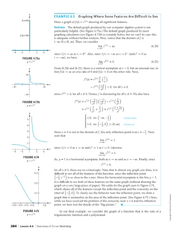
Solution The default graph produced by our computer algebra system is not
particularly helpful. (See Figure 4.73a.) The default graph produced by most
2.5e+08 graphing calculators (see Figure 4.73b) is certainly better, but we can’t be sure this
is adequate without further analysis. First, notice that the domain of f is
(−∞, 0) ∪ (0, ∞). Thus, we consider
lim e 1∕x =∞, (6.20)
x→0 +
x
-4 -2 2 4 + −
t
since 1∕x → ∞ as x → 0 . Also, since 1∕x → −∞ as x → 0 (and e → 0 as
FIGURE 4.73a t → −∞), we have
y = e 1∕x lim e 1∕x = 0. (6.21)
x→0 −
y From (6.20) and (6.21), there is a vertical asymptote at x = 0, but an unusual one, in
that f(x) → ∞ on one side of 0 and f(x) → 0 on the other side. Next,
10 ( )
′
f (x) = e 1∕x d 1
dx x
x 1∕x −1 )
(
-10 10 = e < 0, for all x ≠ 0,
x 2
-10 since e 1∕x > 0, for all x ≠ 0. Hence, f is decreasing for all x ≠ 0. We also have
(
′′
FIGURE 4.73b f (x) = e 1∕x −1 )( −1 ) + e 1∕x ( x 2 3 )
2
2
x
x
y = e 1∕x ( 1 2 ) ( )
= e 1∕x 4 + 3 = e 1∕x 1 + 2x
4
y x x x
( )
⎧ < 0, on −∞, − 1 Concave down.
5 ⎪ 2
( )
1
⎨ − , 0
4 ⎪ > 0, on 2 ∪ (0, ∞). Concave up.
⎩
1
3 Since x = 0 is not in the domain of f, the only inflection point is at x =− . Next,
note that 2
2
lim e 1∕x = 1,
x→∞
1
t
since 1∕x → 0 as x → ∞ and e → 1 as t → 0. Likewise,
x
-4 -2 2 4 lim e 1∕x = 1.
x→−∞
FIGURE 4.74
y = e 1∕x So, y = 1 is a horizontal asymptote, both as x → ∞ and as x → −∞. Finally, since
e 1∕x > 0,
y
for all x ≠ 0, there are no x-intercepts. Note that in almost any graph you draw, it is
0.3 difficult to see all of the features of the function, since the inflection point
( )
1
− ,e −2 is so close to the x-axis. Since the horizontal asymptote is the line y = 1,
2
it is difficult to see both of these features on the same graph (without drawing the
0.2
graph on a very large piece of paper). We settle for the graph seen in Figure 4.74,
which shows all of the features except the inflection point and the concavity on the
)
(
1
0.1 interval − , 0 . To clearly see the behavior near the inflection point, we draw a
2
graph that is zoomed-in on the area of the inflection point. (See Figure 4.75.) Here,
while we have resolved the problem of the concavity near x = 0 and the inflection
x
-0.8 -0.6 -0.4 -0.2 0.2 point, we have lost the details of the “big picture.” Copyright © McGraw-Hill Education
FIGURE 4.75 In our final example, we consider the graph of a function that is the sum of a
y = e 1∕x trigonometric function and a polynomial.
284 | Lesson 4-6 | Overview of Curve Sketching