Page 71 - u4

P2: OSO/OVY
P1: OSO/OVY
GO01962-Smith-v1.cls
UAE-Math-Grade-12-Vol-1-SE-718383-ch4
4-51 QC: OSO/OVY T1: OSO October 25, 2018 17:24 SECTION 4.6 • • Overview of Curve Sketching 261
′
+ 0 - (3 - x) Looking at the individual factors in f (x), we have the number lines shown in the
3 margin. Thus,
- 0 +
(3 + x) {
-3 ′ > 0, on (−3, 0) ∪ (0, 3) f increasing.
+ 0 + f (x) < 0, on (−∞, −3) ∪ (3, ∞). (6.3)
x 4 f decreasing.
0
- 0 + × + 0 - So, f has a local minimum at x =−3 and a local maximum at x = 3.
f�(x)
-3 0 3 Next, we look at
2
3
4
′′
f (x) = −2x(x ) − (9 − x )(4x ) Quotient rule.
4 2
(x )
3
2
2
−2x [x + (9 − x )(2)]
= Factor out −2x .
3
x 8
2
−2(18 − x )
= Combine terms.
x 5
√ √
2(x − 18)(x + 18)
= . Factor difference of two squares.
x 5
′′
Looking at the individual factors in f (x), we obtain the number lines shown in the
- 0 +
2 ( x - √18) margin. Thus, we have
√18
- 0 + { √ √
( x + √18) > 0, on (− 18, 0) ∪ ( 18, ∞) Concave up.
′′
- √18 f (x) √ √ (6.4)
- 0 + < 0, on (−∞, − 18) ∪ (0, 18). Concave down.
x 5
0
√
- 0 + × - 0 + so that there are inflection points at x =± 18. (Why is there no inflection point at
f��(x)
- √18 0 √18 x = 0?)
To determine the limiting behavior as x → ±∞, we consider
2
lim f(x) = lim x − 3
x→∞ x→∞ x 3
( 1 3 )
= lim − = 0. (6.5)
- 0 + × + 0 - x→∞ x x 3
f�(x)
-3 0 3
- 0 + × - 0 +
f��(x) Likewise, we have lim f(x) = 0. (6.6)
- √18 0 √18 x→−∞
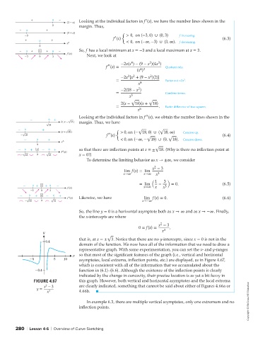
So, the line y = 0 is a horizontal asymptote both as x → ∞ and as x → −∞. Finally,
the x-intercepts are where
2
x − 3
0 = f(x) = ,
y x 3
√
that is, at x =± 3. Notice that there are no y-intercepts, since x = 0 is not in the
0.4
domain of the function. We now have all of the information that we need to draw a
representative graph. With some experimentation, you can set the x- and y-ranges
x so that most of the significant features of the graph (i.e., vertical and horizontal
-5 5 10 asymptotes, local extrema, inflection points, etc.) are displayed, as in Figure 4.67,
which is consistent with all of the information that we accumulated about the
-0.4 function in (6.1)–(6.6). Although the existence of the inflection points is clearly
indicated by the change in concavity, their precise location is as yet a bit fuzzy in
FIGURE 4.67 this graph. However, both vertical and horizontal asymptotes and the local extrema
2
x − 3 are clearly indicated, something that cannot be said about either of Figures 4.66a or
y =
x 3 4.66b.
In example 6.3, there are multiple vertical asymptotes, only one extremum and no Copyright © McGraw-Hill Education
inflection points.

280 | Lesson 4-6 | Overview of Curve Sketching