Page 572 - Microeconomics, Fourth Edition

c13marketstructureandcompetition.qxd 8/2/10 8:19 PM Page 546

546 CHAPTER 13 MARKET STRUCTURE AND COMPETITION
Wow, Samsung has committed to produce 45 units of output; that’s a lot! With that much
output, the market price can’t be any higher than $55, and it would be that high only if we
didn’t produce anything! [P 100 45 55]. That puts us in a somewhat difficult posi-
tion. If we produce the same quantity of output as Samsung, or anything even close to it,
the market price is going to be really low, which is bad news for us. Frankly, Samsung
hasn’t given us very much “wiggle room” to work with here. The best thing for us to do is
to be somewhat conservative in our output choice; sure, we don’t get as much market share
that Samsung has, but at least we keep the market price at a reasonably decent level. Those
guys over at Samsung, by getting the jump on us and moving first, have really boxed us in!
The Stackelberg model of oligopoly is a particular example of a sequential game,
one in which one player in the game moves before the other players do. We will study
sequential games in Chapter 14, and we will see that there can be a strategic value as-
sociated with the ability to be the first mover in the game.

13.3 In some industries, a single company with an overwhelming share of the market—
DOMINANT what economists call a dominant firm—competes against many small producers, each
FIRM of whom has a small market share. For example, in 2004, General Electric had 71.5
percent of the U.S. lightbulb market. The next largest competitor, Osram Sylvania,
MARKETS had just 7.4 percent. 17 During prior periods, U.S. Steel was the dominant firm in the
U.S. steel industry, and Alcoa was the dominant firm in the aluminum industry.
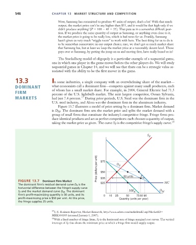
Figure 13.7 illustrates a model of price setting by a dominant firm. Market demand
is D M . The dominant firm sets the market price and splits the market demand with a
group of small firms that constitute the industry’s competitive fringe. Fringe firms pro-
duce identical products and act as perfect competitors: each chooses a quantity of output,
taking the market price as given. The curve S F is the competitive fringe’s supply curve. 18

S F

Price (dollars per unit) $75 D R

$50

FIGURE 13.7 Dominant Firm Market $35 80 units A
$25 MC
The dominant firm’s residual demand curve D R is the
horizontal difference between the fringe’s supply curve D
S F and the market demand curve D M . The dominant MR R M
firm’s profit-maximizing quantity is 50 units, and its 0 10 25 50 75 80 90
profit-maximizing price is $50 per unit. At this price, Quantity (units per year)
the fringe supplies 25 units.

17 U.S. Business Reporter, Market Research, http://www.usbrn.com/mrktdetail2.asp?MarketID
MRK364105 (accessed January 1, 2007).
18 With a fixed number of fringe firms, S F is the horizontal sum of fringe marginal cost curves. The vertical
intercept of S F thus shows the minimum price at which a fringe firm would supply output.