Page 573 - Microeconomics, Fourth Edition

c13marketstructureandcompetition.qxd 7/30/10 1:57 PM Page 547

13.3 DOMINANT FIRM MARKETS 547
The dominant firm’s problem is to find a price that maximizes its profits, taking
into account how that price affects the competitive fringe’s supply. To solve this problem,
, which will tell us
we need to identify the dominant firm’s residual demand curve D R
how much the dominant firm can sell at different prices. We derive D by subtracting
R
the fringe’s supply from the market demand at each price. For example, at a price of
$35, market demand is 90 units, and the price-taking fringe would supply 10 units.
The dominant firm’s residual demand at a price of $35 is thus 80 units. Point A is thus
one point on D . By identifying the horizontal distance between D M and S at every
R
F
price, we can trace out the full residual demand curve. At prices less than $25 per unit,
fringe firms will not supply output, and the dominant firm’s residual demand curve
coincides with the market demand curve. At $75, the dominant firm’s residual demand
shrinks to zero, and fringe firms satisfy the entire market demand.
The dominant firm finds its optimal quantity and price by equating the marginal
revenue MR associated with the residual demand curve to its marginal cost MC ($25
R
in Figure 13.7). We see that the dominant firm’s optimal quantity is 50 units per year,
with the profit-maximizing price of $50 per unit. We use the residual demand curve
rather than the market demand curve to determine the price because it is the residual
demand curve that tells us how much the dominant firm can sell at various market prices.
At a price of $50, market demand is 75 units per year, and the competitive fringe
supplies 25 units. By setting a price of $50, which is twice as high as the minimum
price of $25 at which fringe firms would be willing to supply output, the dominant
firm creates a price umbrella that allows some fringe firms to operate profitably. And
of course, as we have just shown, this price maximizes profit for the dominant firm,
which earns a profit equal to ($50 $25) 50, or $1,250 per year.
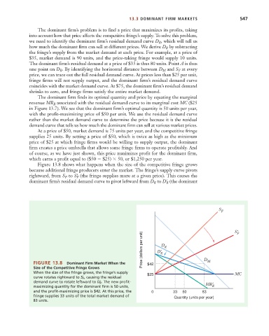
Figure 13.8 shows what happens when the size of the competitive fringe grows
because additional fringe producers enter the market. The fringe’s supply curve pivots
rightward, from S to S¿ F (the fringe supplies more at a given price). This causes the
F
dominant firm’s residual demand curve to pivot leftward from D to D¿ R (the dominant
R

S F

S' F
Price (dollars per unit) D' R D R

FIGURE 13.8 Dominant Firm Market When the $42 D M
Size of the Competitive Fringe Grows
When the size of the fringe grows, the fringe’s supply $25 MC
curve rotates rightward to S F , causing the residual
demand curve to rotate leftward to D R . The new profit- MR'
maximizing quantity for the dominant firm is 50 units, R
and the profit-maximizing price is $42. At this price, the 0 33 50 83
fringe supplies 33 units of the total market demand of Quantity (units per year)
83 units.