Page 682 - Microeconomics, Fourth Edition

c16GeneralEquilibriumTheory.qxd 8/16/10 9:13 PM Page 656

656 CHAPTER 16 GENERAL EQUILIBRIUM THEORY
Suppose, now, that the price of energy is P per unit, while the price of food is P .
x
y
When a household maximizes its utility, it takes these prices and input prices as fixed.
The utility-maximization problems for households are thus:
maxU (x, y), subject to: P x P y I (w, r)
x
W
y
W
(x, y)
max U (x, y), subject to: P x P y I (w, r)
y
B
x
B
(x, y)
where I (w, r) and I (w, r) signify that household incomes depend on the returns that
B
W
households receive from selling their labor and their capital and that these returns
depend on the prices of labor and capital, w and r.
The solutions to these utility-maximization problems yield the optimality con-
ditions that we discussed in Chapter 4:
P x P x
MRS W and MRS B (16.1)
x, y
x, y
P y P y
That is, each household maximizes utility by equating its marginal rate of substitution
of x for y with the ratio of the price of x to the price of y. These optimality conditions,
along with the budget constraints, can be solved for the demand curves for each
household, which depend on the prices and household income.
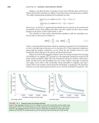
Figure 16.5 shows the aggregate demand curves for energy and food for each type
of household. For example, D W in panel (a) is the aggregate demand for energy by all
x
white-collar households, while D B x is the demand for energy by all blue-collar house-
holds. (In this section and throughout the rest of this chapter, subscripts on demand
and supply curves refer to the commodity being demanded or supplied, and super-
scripts refer to the people or firms doing the demanding or supplying.) We find these
demand curves by summing the demand curves of all the individual households. The

$1 D x 0.80 D y
$1
Price of energy (dollars per unit) 0.60 D x W Price of food (dollars per unit) 0.60 D y W
0.80

0.40
0.40
B
D
0.20
0 5,000 x 10,000 15,000 20,000 0.20 0 D y B 5,000 10,000 15,000 20,000
Quantity of energy (units per year) Quantity of food (units per year)
(a) Energy market (b) Food market

FIGURE 16.5 Demand Curves for Energy and Food
Panel (a): The aggregate demand curves for energy for white-collar households and blue-collar house-
W B W B
holds are D x and D x . The market demand curve for energy (D x ) is the horizontal sum of D x and D x .
Panel (b): The aggregate demand curves for food for white-collar households and blue-collar house-
W B W B
holds are D y and D y . The market demand curve for food (D y ) is the horizontal sum of D y and D y .