Page 684 - Microeconomics, Fourth Edition

c16GeneralEquilibriumTheory.qxd 8/16/10 9:13 PM Page 658

658 CHAPTER 16 GENERAL EQUILIBRIUM THEORY

Price of labor (dollars per unit) 0.5 Price of capital (dollars per unit) 0.5

$1
$1

D D x L D K
D L y L D K y D K x
0 2000 4000 6000 8000 0 2000 4000 6000 8000
Quantity of labor (units) Quantity of capital (units)
(a) Labor market (b) Capital market

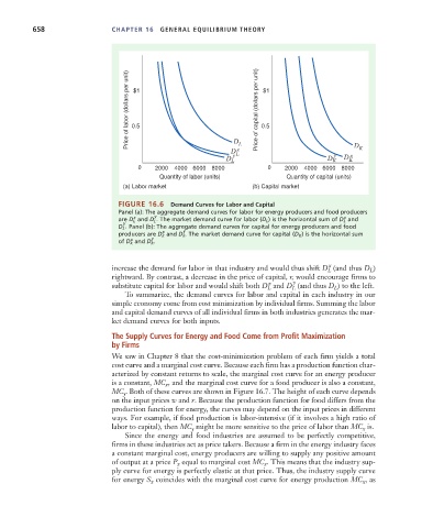
FIGURE 16.6 Demand Curves for Labor and Capital
Panel (a): The aggregate demand curves for labor for energy producers and food producers
x y x
are D L and D . The market demand curve for labor (D L ) is the horizontal sum of D L and
L
y
D L . Panel (b): The aggregate demand curves for capital for energy producers and food
x y
producers are D k and D k . The market demand curve for capital (D K ) is the horizontal sum
x y
of D k and D k .
increase the demand for labor in that industry and would thus shift D L x (and thus D L )
rightward. By contrast, a decrease in the price of capital, r, would encourage firms to
substitute capital for labor and would shift both D L x and D L y (and thus D L ) to the left.
To summarize, the demand curves for labor and capital in each industry in our
simple economy come from cost minimization by individual firms. Summing the labor
and capital demand curves of all individual firms in both industries generates the mar-
ket demand curves for both inputs.

The Supply Curves for Energy and Food Come from Profit Maximization
by Firms
We saw in Chapter 8 that the cost-minimization problem of each firm yields a total
cost curve and a marginal cost curve. Because each firm has a production function char-
acterized by constant returns to scale, the marginal cost curve for an energy producer
is a constant, MC x , and the marginal cost curve for a food producer is also a constant,
MC y . Both of these curves are shown in Figure 16.7. The height of each curve depends
on the input prices w and r. Because the production function for food differs from the
production function for energy, the curves may depend on the input prices in different
ways. For example, if food production is labor-intensive (if it involves a high ratio of
labor to capital), then MC y might be more sensitive to the price of labor than MC x is.
Since the energy and food industries are assumed to be perfectly competitive,
firms in these industries act as price takers. Because a firm in the energy industry faces
a constant marginal cost, energy producers are willing to supply any positive amount
of output at a price P x equal to marginal cost MC x . This means that the industry sup-
ply curve for energy is perfectly elastic at that price. Thus, the industry supply curve
for energy S x coincides with the marginal cost curve for energy production MC x , as