Page 689 - Microeconomics, Fourth Edition

c16GeneralEquilibriumTheory.qxd 8/16/10 9:13 PM Page 663

16.2 GENERAL EQUILIBRIUM ANALYSIS: MANY MARKETS 663

An industry that was particularly affected by the income effects were becoming important to consumer
rise in oil prices was automobiles. In 2008, sales of demand, as sales of cars, both imported and domestic,
sport-utility vehicles (SUVs) declined 25 percent. At the began to decline considerably as well. In addition, the
same time, domestic car sales fell 7 percent, imported fall in demand for SUVs, trucks, and cars affected the
car sales rose 10 percent, but sales of imported light labor market. Seasonally adjusted employment in the
trucks fell 22 percent. These results strongly suggest motor vehicle and parts industries declined by 125,000
that substitution effects were more important than over this period. Of course, that unemployment fur-
income effects. Consumers were shifting from vehicles ther reduced demand for many consumer goods, and
with low- fuel efficiency, such as SUVs and trucks, and increasing problems in the housing market (especially
toward smaller and more fuel-efficient cars (imported in cities such as Detroit in which vehicle manufacturing
cars tend to fit into those categories). However, by the is an important part of the local economy) contributed
end of 2008 the severity of the recession meant that further to the recession.

The general equilibrium analysis in Figure 16.9 highlights the relationship between
the scarcity of factors of production, the relative prices of those factors, and the distribu-
tion of income in the economy. In the economy in Figure 16.9, the aggregate supply of
capital is much less than the aggregate supply of labor (i.e., S is closer to its vertical axis
K
than is S ). As a result, the price of capital services exceeds the price of labor (i.e., capital
L
services trade at a price premium compared to labor services). This, in turn, allows the
providers of capital inputs—the white-collar households in our economy—to earn higher
incomes than the providers of labor inputs—primarily blue-collar households.
Learning-By-Doing Exercise 16.2 shows how to write the supply-equals-demand
conditions that determine a general equilibrium for our simple economy.

LEARNING-BY-DOING EXERCISE 16.2
S
D
E
Finding the Conditions for a General Equilibrium with Four Markets
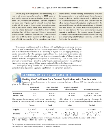
Suppose that the households in the simple economy depicted in Figure 16.9 have the characteristics
given in the following table:
Number of Labor Supplied Capital Supplied
Households per Household per Household Household Income

Blue Collar 100 60 units 0 units I B (w, r) 60w
White Collar 100 10 units 50 units I W (w, r) 10w 50r

Also suppose that the supply and demand curves for the table, where X is the overall quantity of energy de-
markets in this economy are as shown in the following manded and Y is the overall quantity of food demanded: 4

Energy Food Labor Capital
1 2 1 1
Supply P x w r 3 P y w r 2 L 7000* K 5000*
3
2
2 1 1 1
50I W 75I B 50I W 25I B X r 3 Y r 2 2X w 3 Y w 2
Demand P x P Y L a b a b K a b a b
X Y 3 w 2 w 3 r 2 r
*Based on supply per household, as shown in the table showing the number of households above [L (100 10)
(100 60) 7000; K (100 50) (100 0) 5000].
4 In the Appendix, we show how these curves are derived from the cost-minimization problems of individ-
ual firms and the utility-maximization problems of individual households.