Page 124 - Fiber Optic Communications Fund

Lasers 105

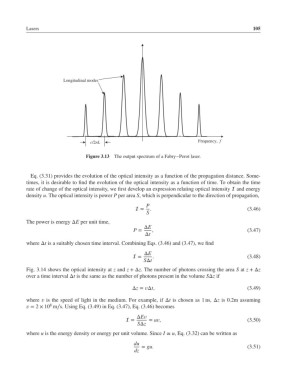
Longitudinal modes

c/2nL Frequency, f

Figure 3.13 The output spectrum of a Fabry–Perot laser.

Eq. (3.31) provides the evolution of the optical intensity as a function of the propagation distance. Some-
times, it is desirable to find the evolution of the optical intensity as a function of time. To obtain the time
rate of change of the optical intensity, we first develop an expression relating optical intensity  and energy
density u. The optical intensity is power P per area S, which is perpendicular to the direction of propagation,

P
 = . (3.46)
S
The power is energy ΔE per unit time,
ΔE
P = , (3.47)
Δt
where Δt is a suitably chosen time interval. Combining Eqs. (3.46) and (3.47), we find

ΔE
 = . (3.48)
SΔt
Fig. 3.14 shows the optical intensity at z and z +Δz. The number of photons crossing the area S at z +Δz
over a time interval Δt is the same as the number of photons present in the volume SΔz if

Δz = Δt, (3.49)
where is the speed of light in the medium. For example, if Δt is chosen as 1 ns, Δz is 0.2m assuming
8
= 2 × 10 m∕s. Using Eq. (3.49) in Eq. (3.47), Eq. (3.46) becomes
ΔE
 = = u, (3.50)
SΔz
where u is the energy density or energy per unit volume. Since I ∝ u, Eq. (3.32) can be written as
du
= gu. (3.51)
dz