Page 184 - Fiber Optic Communications Fund

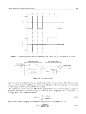
Optical Modulators and Modulation Schemes 165

0 1 0 1 1 1
+1 V

u in (t) 0 t

–1 V

+2 V

u out (t) 0 t

–2 V

Figure 4.27 Duobinary encoding. The data in the interval −T < t < 0of u (t) is assumed to be ‘0’ (−1 V).
b
in
Differential coding Add-and-delay filter
Polar NRZ data
Duobinary data
b'(t) +
b(t) m(t)
Delay
T
b
Delay T b
Figure 4.28 Duobinary encoder.

leads to a sample value of ±2 V at kT . This significantly simplifies the decision rule: if the absolute sample
b
value is ≤ 1 V, ‘1’ is transmitted. Otherwise, ‘0’ is transmitted. Fig. 4.28 shows the realization of a duobinary
encoder and Fig. 4.29 an example of duobinary encoding.
We can introduce a known amount of ISI such that a pulse in the 0th bit slot interferes only with a pulse in
the first bit slot and does not interfere with pulses in other bit slots at sampling instants t = nT , where n is
b
an integer. Such a pulse can be described by
{
1 n = 0, 1
p(nT )= . (4.90)
b
0 otherwise
An example of a pulse satisfying the requirement of Eq. (4.90) is a Nyquist pulse [1], [7],
sin (Bt)
p(t)= , (4.91)
Bt(1 − Bt)