Page 322 - Fiber Optic Communications Fund

Transmission System Design 303

1.4 1.4
1.2 1.2

1 I 1 1 I 1
Current, I 0.8 Current, I 0.8

0.6
0.6
0.4 0.4
0.2 0.2
I
0 0 0 I
0.5 0 0.5 1 0.5 0 0.5 1 0
Time (s) x 10 –10 Time (s) x 10 –10
(a) At the transmitter (b) At the receiver
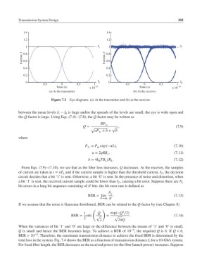
Figure 7.3 Eye diagrams. (a) At the transmitter and (b) at the receiver.

between the mean levels I − I is large and/or the spreads of the levels are small, the eye is wide open and
0
1
the Q-factor is large. Using Eqs. (7.4)–(7.8), the Q-factor may be written as
RP 1r
Q = √ , (7.9)
√
aP + b + b
1r
where
P = P exp (−L), (7.10)
1r
in
a = 2qRB , (7.11)
e
b = 4k TB ∕R . (7.12)
L
e
B
From Eqs. (7.9)–(7.10), we see that as the fiber loss increases, Q decreases. At the receiver, the samples
of current are taken at t = nT and if the current sample is higher than the threshold current, I , the decision
b T
circuit decides that a bit ‘1’ is sent. Otherwise, a bit ‘0’ is sent. In the presence of noise and distortion, when
a bit ‘1’ is sent, the received current sample could be lower than I , causing a bit error. Suppose there are N
T e
bit errors in a long bit sequence consisting of N bits; the bit error rate is defined as
N e
BER = lim . (7.13)
N→∞ N
If we assume that the noise is Gaussian distributed, BER can be related to the Q-factor by (see Chapter 8)
( )
2
1 Q exp(−Q ∕2)
BER = erfc √ ≈ √ . (7.14)
2 2 2Q
When the variances of bit ‘1’ and ‘0’ are large or the difference between the means of ‘1’ and ‘0’ is small,
−9
Q is small and hence the BER becomes large. To achieve a BER of 10 , the required Q is 6. If Q < 6,
−9
BER > 10 . Therefore, the maximum transmission distance to achieve the fixed BER is determined by the
total loss in the system. Fig. 7.4 shows the BER as a function of transmission distance L for a 10-Gb/s system.
For fixed fiber length, the BER decreases as the received power (or the fiber launch power) increases. Suppose