Page 333 - Fiber Optic Communications Fund

314 Fiber Optic Communications

1 0 1 1 1
1
0.9
0.8 0.8
0.7
Power (mW) 0.6 Power (mW) 0.5
0.6

0.4
0.4
0.3
0.2 0.2
0.1
0 0
–2 –1 0 1 2 –3 –2 –1 0 1 2 3
Time (t/T b ) Time (t/T b )
(b) Output
(a) Input
2
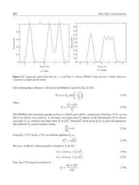
Figure 7.12 Input and output of the fiber. =−21 ps /km, L = 40 km, FWHM = 50 ps, bit rate = 10 Gb/s. Fiber loss
2
is ignored. (a) Input and (b) output.
After propagating a distance L, the power distribution is given by Eq. (2.161),
( )
t 2
P(t, L)= P exp − , (7.92)
in
T 2
L
where
2 2
4
T + L
2
0
2
T = . (7.93)
L 2
T
0
The FWHM at the transmitter and the receiver is 1.665T and 1.665T , respectively. From Eq. (7.93), we see
0 L
2
that if we choose very small T , T becomes very large since T appears in the denominator. If we choose
0 L 0
4
2 2
very large T , T could become large when T ≫ L . Therefore, for the given | |L, T has to be optimized.
0
2
0
L
2
0
The optimum T can be found by setting
0
dT L
= 0. (7.94)
dT
0
Using Eq. (7.93 ) in Eq. (7.94), we find the optimum T as
0
opt √
T = L. (7.95)
2
0
The r.m.s. width of a Gaussian pulse is related to T by [4]
0
√
(z = 0) ≡ = T ∕ 2, (7.96)
0 0
√
(z = L) ≡ = T ∕ 2. (7.97)
L
L
Now, Eq. (7.93) may be rewritten as
4
2 2
4 + L
2
0
2
= . (7.98)
L 2
4
0