Page 60 - Fiber Optic Communications Fund

Optical Fiber Transmission 41

Power (arb. units)

T B t
(a)
Power (arb. units)

t
ΔT
(b)

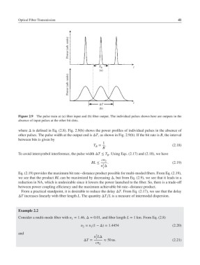
Figure 2.9 The pulse train at (a) fiber input and (b) fiber output. The individual pulses shown here are outputs in the
absence of input pulses at the other bit slots.

where Δ is defined in Eq. (2.8). Fig. 2.9(b) shows the power profiles of individual pulses in the absence of
other pulses. The pulse width at the output end is ΔT, as shown in Fig. 2.9(b). If the bit rate is B, the interval
between bits is given by
1
T = . (2.18)
B
B
To avoid intersymbol interference, the pulse width ΔT ≤ T . Using Eqs. (2.17) and (2.18), we have
B
cn
BL ≤ 2 . (2.19)
2
n Δ
1
Eq. (2.19) provides the maximum bit rate–distance product possible for multi-moded fibers. From Eq. (2.19),
we see that the product BL can be maximized by decreasing Δ, but from Eq. (2.9), we see that it leads to a
reduction in NA, which is undesirable since it lowers the power launched to the fiber. So, there is a trade-off
between power coupling efficiency and the maximum achievable bit rate–distance product.
From a practical standpoint, it is desirable to reduce the delay ΔT. From Eq. (2.17), we see that the delay
ΔT increases linearly with fiber length L. The quantity ΔT∕L is a measure of intermodal dispersion.

Example 2.2
Consider a multi-mode fiber with n = 1.46, Δ= 0.01, and fiber length L = 1 km. From Eq. (2.8)
1
n = n (1 −Δ) = 1.4454 (2.20)
2 1
and
2
n LΔ
1
ΔT = ≈ 50 ns. (2.21)
cn
2