Page 62 - Fiber Optic Communications Fund

Optical Fiber Transmission 43

n
n 1 1 n 1

n(r) n(r) n(r)

n n
n 2 2 2
a r a r a r
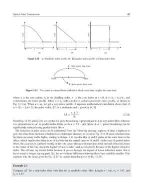
(a) (b) (c)
Figure 2.11 (a) Parabolic index profile. (b) Triangular index profile. (c) Step-index fiber.

A : High speed, long route

Home Office
B : Low speed, short route

Figure 2.12 Two paths to connect home and office which could take roughly the same time.

where a is the core radius, n is the cladding index, n is the core index at r = 0, Δ=(n − n )∕n , and
2 1 1 2 1
determines the index profile. When = 2, such a profile is called a parabolic index profile,asshown in
Fig. 2.11(a). When =∞, we get a step-index profile. A rigorous mathematical calculation shows that, if
= 2(1 − Δ)(≈ 2), the pulse width, ΔT, is a minimum and is given by [4, 5]
2
n Δ L
1
ΔT = . (2.24)
8c
From Eqs. (2.23) and (2.24), we see that the pulse broadening is proportional to Δ in step-index fibers whereas
2
it is proportional to Δ in graded-index fibers (with = 2(1 −Δ)). Since Δ ≪ 1, pulse broadening can be
significantly reduced using graded-index fibers.
The reduction in pulse delay can be understood from the following analogy: suppose A takes a highway to
go to the office from his home which is faster, but longer distance, as shown in Fig. 2.12. B takes a shorter route
but there are many traffic lights, leading to delays. It is possible that A and B arrive at the same time to the
office, which implies that there is no delay between the arrival times of A and B. In the case of graded-index
fibers, the axial ray is confined mostly to the core center (because it undergoes total internal reflection closer
to the center of the core due to the higher refractive index) and travels slowly because of the higher refractive
index. The off-axis ray travels faster because it passes through the region of lower refractive index. But it
has to travel a longer zig-zag path. So, the arrival time difference between these rays could be smaller. This
explains why the delay given by Eq. (2.24) is smaller than that given by Eq. (2.23).

Example 2.3
Compare ΔT for a step-index fiber with that for a parabolic-index fiber. Length = 1km, n = 1.47, and
1
n = 1.45.
2