Page 112 - Computer Graphics Handout

3.6.5 Interpolation
Although we have specified colors for the vertices of the cube, the graphics system must decide
how to use this information to assign colors to points inside the polygon. There are many ways to
use the colors of the vertices to fill in, or interpolate, colors across a polygon. Probably the most
common method used in computer graphics is based on the barycentric coordinate
representation of triangles that we introduced in Section 3.1. One of the major reasons for this
approach is that triangles are the key object that we work with in rendering.
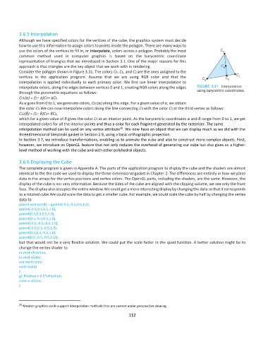
Consider the polygon shown in Figure 3.31. The colors C0, C1, and C2 are the ones assigned to the
vertices in the application program. Assume that we are using RGB color and that the
interpolation is applied individually to each primary color. We first use linear interpolation to
interpolate colors, along the edges between vertices 0 and 1, creating RGB colors along the edges
through the parametric equations as follows:
C01(α) = (1− α)C0+ αC1.
As α goes from 0 to 1, we generate colors, C01(α) along this edge. For a given value of α, we obtain
the color C3.We can now interpolate colors along the line connecting C3 with the color C2 at the third vertex as follows:
C32(β) = (1− β)C3+ βC2,
which for a given value of β gives the color C4 at an interior point. As the barycentric coordinates α and β range from 0 to 1, we get
interpolated colors for all the interior points and thus a color for each fragment generated by the rasterizer. The same
20
interpolation method can be used on any vertex attribute . We now have an object that we can display much as we did with the
threedimensional Sierpinski gasket in Section 2.9, using a basic orthographic projection.
In Section 3.7, we introduce transformations, enabling us to animate the cube and also to construct more complex objects. First,
however, we introduce an OpenGL feature that not only reduces the overhead of generating our cube but also gives us a higher-
level method of working with the cube and with other polyhedral objects.

3.6.6 Displaying the Cube
The complete program is given in Appendix A. The parts of the application program to display the cube and the shaders are almost
identical to the the code we used to display the three-dimensional gasket in Chapter 2. The differences are entirely in how we place
data in the arrays for the vertex positions and vertex colors. The OpenGL parts, including the shaders, are the same. However, the
display of the cube is not very informative. Because the sides of the cube are aligned with the clipping volume, we see only the front
face. The display also occupies the entire window.We could get a more interesting display by changing the data so that it corresponds
to a rotated cube.We could scale the data to get a smaller cube. For example, we could scale the cube by half by changing the vertex
data to
point4 vertices[8] = {point4(-0.5,-0.5,0.5,1.0),
point4(-0.5,0.5,0.5,1.0),
point4(0.5,0.5,0.5,1.0),
point4(0.5,-0.5,0.5,1.0),
point4(-0.5,-0.5,-0.5,1.0),
point4(-0.5,0.5,-0.5,1.0),
point4(0.5,0.5,-0.5,1.0),
point4(0.5,-0.5,-0.5,1.0)};
but that would not be a very flexible solution. We could put the scale factor in the quad function. A better solution might be to
change the vertex shader to
in vec4 vPosition;
in vec4 vColor;
out vec4 color;
void main()
{
gl_Position = 0.5*vPosition;
color = vColor;
}

20 Modern graphics cards support interpolation methods that are correct under perspective viewing.
112