Page 113 - Computer Graphics Handout

Note that we also changed the vertex shader to use input data in four-dimensional homogeneous coordinates. We also can simplify
the fragment shader to
in vec4 color;
out vec4 fragColor;
void main()
{
fragColor = color;
}
Rather than looking at these ad hoc approaches, we will develop a transformation capability that will enable us to rotate, scale, and
translate data either in the application or in the shaders. We will also examine in greater detail how we convey data among the
application and shaders that enable us to carry out transformations in the GPU and alter transformations dynamically.

3.7 AFFINE TRANSFORMATIONS

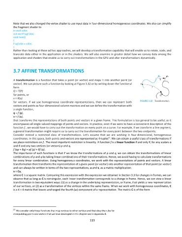
A transformation is a function that takes a point (or vector) and maps it into another point (or
vector). We can picture such a function by looking at Figure 3.32 or by writing down the functional
form
Q = T(P)
for points, or
v = R(u)
for vectors. If we use homogeneous coordinate representations, then we can represent both
vectors and points as four-dimensional column matrices and we can define the transformation with
a single function,
q = f (p),
v = f (u),
that transforms the representations of both points and vectors in a given frame. This formulation is too general to be useful, as it
encompasses all single-valued mappings of points and vectors. In practice, even if we were to have a convenient description of the
function f , we would have to carry out the transformation on every point on a curve. For example, if we transform a line segment,
a general transformation might require us to carry out the transformation for every point between the two endpoints.
Consider instead a restricted class of transformations. Let’s assume that we are working in four-dimensional, homogeneous
21
coordinates. In this space, both points and vectors are represented as 4-tuples . We can obtain a useful class of transformations if
we place restrictions on f . The most important restriction is linearity. A function f is a linear function if and only if, for any scalars α
and β and any two vertices (or vectors) p and q,
f (αp + βq) = αf (p) + βf (q).
The importance of such functions is that if we know the transformations of p and q, we can obtain the transformations of linear
combinations of p and q by taking linear combinations of their transformations. Hence, we avoid having to calculate transformations
for every linear combination. Using homogeneous coordinates, we work with the representations of points and vectors. A linear
transformation then transforms the representation of a given point (or vector) into another representation of that point (or vector)
and can always be written in terms of the two representations, u and v, as a matrix multiplication:
v = Cu,
where C is a square matrix. Comparing this expression with the expression we obtained in Section 3.3 for changes in frames, we can
observe that as long as C is nonsingular, each linear transformation corresponds to a change in frame. Hence, we can view a linear
transformation in two equivalent ways: (1) as a change in the underlying representation, or frame, that yields a new representation
of our vertices, or (2) as a transformation of the vertices within the same frame. When we work with homogeneous coordinates, C
is a 4 × 4 matrix that leaves unchanged the fourth (w) component of a representation. The matrix C is of the form

21
We consider only those functions that map vertices to other vertices and that obey the rules for
manipulating points and vectors that we have developed in this chapter and in Appendix B.
113