Page 29 - manual_V5_11_9_2018_Html5

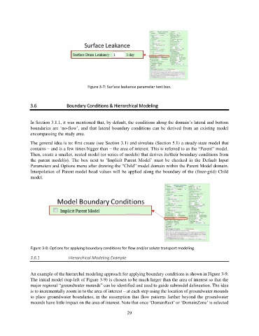
Figure 3-7: Surface leakance parameter text box.

3.6 Boundary Conditions & Hierarchical Modeling

In Section 3.1.1, it was mentioned that, by default, the conditions along the domain’s lateral and bottom
boundaries are ‘no-flow’, and that lateral boundary conditions can be derived from an existing model
encompassing the study area.
The general idea is to: first create (see Section 3.1) and simulate (Section 5.1) a steady-state model that
contains – and is a few times bigger than – the area of interest. This is referred to as the “Parent” model.
Then, create a smaller, nested model (or series of models) that derives its/their boundary conditions from
the parent model(s). The box next to ‘Implicit Parent Model’ must be checked in the Default Input
Parameters and Options menu after drawing the “Child” model domain within the Parent Model domain.
Interpolation of Parent model head values will be applied along the boundary of the (finer-grid) Child
model.

Figure 3-8: Options for applying boundary conditions for flow and/or solute transport modeling.

3.6.1 Hierarchical Modeling Example

An example of the hierarchal modeling approach for applying boundary conditions is shown in Figure 3-9.
The initial model (top-left of Figure 3-9) is chosen to be much larger than the area of interest so that the
major regional “groundwater mounds” can be identified and used to guide submodel delineation. The idea
is to incrementally zoom in to the area of interest – at each step using the location of groundwater mounds
to place groundwater boundaries, in the assumption that flow patterns further beyond the groundwater
mounds have little impact on the area of interest. Note that once ‘DomanRect’ or ‘DomainZone’ is selected

29