Page 39 - ASBIRES-2017_Preceedings

Dharamasooriya, Ekanayake & Appuhamy

Table 4: Level of normative commitment
Autocorrelation Function for loss%
Level Frequency Percentage/ (%) (with 5% significance limits for the autocorrelations)
1.0
High 20 40 0.8
0.6
0.4
Moderate 6 12 0.2
0.0
Low 24 48 Autocorrelation -0.2
-0.4
-0.6
As seen in Table 4, nearly 50 percent -0.8
of employees’ normative commitment to the -1.0 1 10 20 30 40 50 60 70 80 90
organization was low. On the other hand, 40 Lag
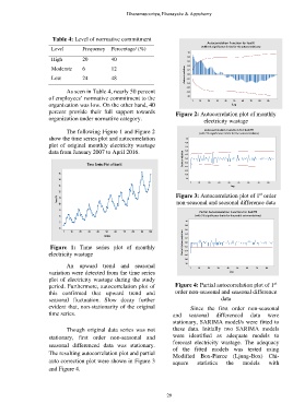
percent provide their full support towards Figure 2: Autocorrelation plot of monthly
organization under normative category. electricity wastage

Autocorrelation Function for Sediff1
The following Figure 1 and Figure 2 (with 5% significance limits for the autocorrelations)
show the time series plot and autocorrelation 1.0
plot of original monthly electricity wastage 0.8
0.6
data from January 2007 to April 2016. 0.4
Autocorrelation 0.0
0.2
Time Series Plot of loss% -0.2
-0.4
-0.6
15 -0.8
14 -1.0
1 10 20 30 40 50 60 70 80
13 Lag
12 st
loss% 11 Figure 3: Autocorrelation plot of 1 order
10 non-seasonal and seasonal difference data
9
Partial Autocorrelation Function for Sediff1
8 (with 5% significance limits for the partial autocorrelations)
7 1.0
0.8
6
1 10 20 30 40 50 60 70 80 90 100 0.6
Index 0.4
0.2
0.0
Figure 1: Time series plot of monthly Partial Autocorrelation -0.2
electricity wastage -0.4
-0.6
-0.8
An upward trend and seasonal -1.0 1 10 20 30 40 50 60 70 80
variation were detected from the time series Lag

plot of electricity wastage during the study
st
period. Furthermore, autocorrelation plot of Figure 4: Partial autocorrelation plot of 1
this confirmed that upward trend and order non-seasonal and seasonal difference
seasonal fluctuation. Slow decay further data
evident that, non-stationarity of the original Since the first order non-seasonal
time series. and seasonal differenced data were
stationary, SARIMA model/s were fitted to
Though original data series was not these data. Initially two SARIMA models
stationary, first order non-seasonal and were identified as adequate models to
seasonal differenced data was stationary. forecast electricity wastage. The adequacy
of the fitted models was tested using
The resulting autocorrelation plot and partial Modified Box-Pierce (Ljung-Box) Chi-
auto correction plot were shown in Figure 3 square statistics the models with
and Figure 4.

29