Page 43 - ASBIRES-2017_Preceedings

Kaushalya & Francisco

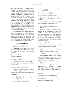
cases from June 2002 to September 2012. r k (2)
r
The proposed model is only based on the t = 1 √1+2 ∑ r 2 j
k
humidity and temperature and it does not √n
require rainfall measurements take into H :Autocorrelation at lag k is zero.
0
account. Wongkoon, Jaroensutasinee & H :Autocorrelation at lag k is not zero
Jaroensutasinee (2011) studied and 1
identified temporary model to predict Then the null hypothesis (H0) is
Dengue cases in Northeastern Thailand. accepted if
Using the Box Jenkins approach ARIMA
(3,1, 4) was found as the best suitable model |t |<2 , That is autocorrelation at lag k
r k
with the lowest AIC and MAPE value. is zero. Autocorrelation does not exist.
Siriyasatien, Phumee, Ongruk, Jampachaisri
& Kesorn (2016) conducted their study on 3.4 Partial Autocorrelation Function
analysis of significant factors for dengue (PACF)
fever incidence prediction. A partial correlation coefficient is the

The predictive power of the forecasting measure of the relationship between two
model was assessed by (AIC), Bayesian variables when the effect of other variables
information criterion (BIC), and the mean has been removed or been constant.
absolute percentage error (MAPE). The Similarly, the partial autocorrelation (ρ ) is
k k
selected model was with the lowest AIC, the the measure of the relationship between the
lowest BIC, and a small MAPE value stationary time series variables x and x
t
t+k
among all three other competing models. when the adjustment.

3.5 Stationary Time Series
3 METHODOLOGY
A time series is said to be stationary if,
3.1 Augmented Dicky Fuller Test Mean of the time series is stationary

Augmented Dicky Fuller (ADF) test is
t
used to identify whether there is a unit root E(x ) = μ (3)
in a Time Series. Then it tests the null Time series has a constant variance.
hypothesis,
2
Var(x )=σ (4)
t
H :unit root is in the series Autocorrelation depends only on the
0
H :series is stationary time interval(lag). In practice, we use
1
Correlogram to identify the stationarity or
3.2 Phillips Perron Test
non-stationarity of a time series.
Phillip Perron test is also used to
identify whether there is a unit root present 3.6 Differencing
in a time series. In practice, most of the time series are

3.3 Autocorrelation Function(ACF) non-stationary. Therefore, suitable
differencing of data is required to make the
Unknown population autocorrelation is time series stationary. First order non-
estimated by using sample autocorrelation seasonal difference
function. The sample autocorrelation at lag k (∇x )=x -x (5)
is denoted by t t t-1
Second order non-seasonal difference
n-k
∑ (Xt-X ̅ )(Xt+k-X ̅ )
r = t=b 2 (1) (∇x )=∇x -∇x (6)
k
∑ n t=b (Xt-X ̅ ) t t t-1
First order seasonal difference
The test statistic (t ) is given by
r k

33